Data-driven approach for creating synthetic electronic medical records

(1)

R E S E A R C H A R T I C L E

Open Access

Data-driven approach for creating synthetic

electronic medical records

Anna L Buczak

*

, Steven Babin, Linda Moniz

Abstract

Background:New algorithms for disease outbreak detection are being developed to take advantage of full electronic medical records (EMRs) that contain a wealth of patient information. However, due to privacy concerns, even anonymized EMRs cannot be shared among researchers, resulting in great difficulty in comparing the effectiveness of these algorithms. To bridge the gap between novel bio-surveillance algorithms operating on full EMRs and the lack of non-identifiable EMR data, a method for generating complete and synthetic EMRs was developed.

Methods:This paper describes a novel methodology for generating complete synthetic EMRs both for an outbreak illness of interest (tularemia) and for background records. The method developed has three major steps:

1) synthetic patient identity and basic information generation; 2) identification of care patterns that the synthetic patients would receive based on the information present in real EMR data for similar health problems;

3) adaptation of these care patterns to the synthetic patient population.

Results:We generated EMRs, including visit records, clinical activity, laboratory orders/results and radiology orders/ results for 203 synthetic tularemia outbreak patients. Validation of the records by a medical expert revealed problems in 19% of the records; these were subsequently corrected. We also generated background EMRs for over 3000 patients in the 4-11 yr age group. Validation of those records by a medical expert revealed problems in fewer than 3% of these background patient EMRs and the errors were subsequently rectified.

Conclusions:A data-driven method was developed for generating fully synthetic EMRs. The method is general and can be applied to any data set that has similar data elements (such as laboratory and radiology orders and results, clinical activity, prescription orders). The pilot synthetic outbreak records were for tularemia but our approach may be adapted to other infectious diseases. The pilot synthetic background records were in the 4-11 year old age group. The adaptations that must be made to the algorithms to produce synthetic background EMRs for other age groups are indicated.

I. Background I.a Motivation

Despite the current push to adopt electronic medical records (EMRs) as the standard for patient records, research concerned with utilizing all the information in EMRs may be compromised because legal restrictions and privacy concerns limit access to EMRs in academic and industrial research settings to a small number of institutions that have access to the full records. For example, any algorithm designed to work on EMRs can only be tested on a specific set of records so that there

is no consistent set of test data that can be used by all interested parties to compare the efficacy of different algorithms. To avoid compromising patient privacy and hospital proprietary concerns, the intent of the Synthetic Electronic Medical Records Generator (EMERGE) pro-ject is to develop a methodology for creating synthetic EMRs from a set of real EMRs. Using EMERGE, test beds could be synthesized, creating EMRs for both back-ground records and artificial outbreaks or emergencies that are not present in the real data. The availability of a standardized set of test data would allow comparison of different algorithms and procedures that operate on EMRs as well as provide a set of records for the devel-opment of such algorithms.

* Correspondence: [email protected]

Johns Hopkins University Applied Physics Laboratory, 11100 Johns Hopkins Rd, Laurel, MD 20723-6099, USA

(2)

There are privacy and proprietary concerns with the dissemination of medical record data [1]. These con-cerns remain even if it is sanitized or anonymized [2,3] because of the variety of different types and sources of data tied together within the EMR. Even having just the compound of ZIP code, gender, and date of birth has been described as being sufficient for uniquely identify-ing a large percentage of the population of the United States [4]. The development of synthetic EMR data for both background records and injected disease records is thus vital for increased research in the mining of data in EMRs to improve quality of care, detection of health threats, and monitoring for adverse drug effects.

The first EMERGE product provided us with valuable lessons that were used in the methodology described in this paper. This earlier product was a set of synthetic EMRs of infected patients who were exposed to a ficti-tious bioterrorism event, the release of airborne tulare-mia in the restrooms at a sporting event [5]. The synthetic victims (i.e., infected patients) were 4 to 89 years old and included both males and females. The vic-tims’demographics were chosen from the typical demo-graphics of individuals using the luxury boxes at a baseball game. We created synthetic EMRs that reflected the entire timeline of pneumonic tularemia from pro-drome, when present, to severe illness, and that were based upon synthesized models of care using informa-tion from the literature on the progression of the dis-ease, as well as similar cases of flulike illness and progression to pneumonia present in the set of original background EMRs. Unfortunately, the utility of these synthetic EMRs was limited because, although the injected victims were completely synthetic, the ground records were not. Even though these back-ground EMRs were de-identified and date-scrambled via the RBNR algorithm [6], they were considered real enough that they could not be posted on the public health grid [7,8]. In contrast, the completely synthetic EMRs were allowed to be posted. However, the useful-ness of the total set of EMRs as a test data set for out-break detection algorithms was limited to the institutions that had legal and proprietary access to the background data. For this reason, the synthesis of back-ground records became a major part of the EMERGE project. At the time of the creation of this earlier syn-thetic tularemia outbreak, it was not at all clear that the complexity of the records for a background population would lend itself to synthesis.

We tested, analyzed, and refined methods to extract meaningful information from real EMRs to produce syn-thetic EMRs, as well as ways to represent the informa-tion in a mathematically consistent fashion. After this analysis, we devised a three-part method that would allow automation of the synthesis process with as much

fidelity as possible in information content but without compromising details that defined any original patient’s identity. This three-part-method consists of: 1) the synthesis of patient identities; 2) the identification of models-of-care in real EMRs; and 3) the adaptation of models-of-care to the synthetic patients. We will describe the processes in detail both for the set of injected tularemia patients and the set of synthetic back-ground patients. Because the pilot age group for the background records was 4-11 yr olds, we will suggest adaptations to this method that we believe are necessary for the creation of data sets beyond this single age group.

I.b Related Work

There has been considerable research utilizing the infor-mation contained in EMRs. Some recent results occur in bio-surveillance [9-13], screening for reportable dis-ease [14-16] and pharmacovigilance [17,18]. However, there has not been a corresponding increase in the avail-ability of non-identifiable complete EMRs for the devel-opment or test of algorithms that operate on them.

There have been various efforts at de-identification of medical record information, including the Realistic But Not Real (RBNR) project [6], and recent work on identification of clinical notes [19]. Algorithms to de-identify visit records are an active area of research (see, e.g. [20] and references therein) but these algorithms in general do not operate on the entire EMR. As men-tioned before, there is some danger in the widespread dissemination of even anonymized or de-identified data. The main risk is that an individual patient or a particu-lar facility or practitioner could potentially be uniquely identified from the conjunction of different types of information within the EMR, such as age group, gender, ethnic group, race, time of medical encounter, or a rare or unusual-for-age diagnosis. Because the medical infor-mation itself is not altered by anonymization and date-shuffling algorithms, it is possible that some information in the EMR could be used to identify a patient, a practi-tioner, or a facility. Proprietary as well as privacy con-cerns, then, motivate the need to produce synthetic patients that display enough variation in demographic and sanitized medical record information to make iden-tification of the patient and the facility ambiguous.

(3)

does not, at this time, model the clinical timelines of patients with infectious disease or injury.

There are many different models for the spread of infectious disease through a population. From a simple lognormal curve [22-24] through the injection of artifi-cial disease outbreaks in simulated time series [25] to the recent population model for the Models of Infec-tious Disease Agent Study (MIDAS, [26]), they can vary in complexity, scope and purpose. The focus in Project Mimic [25] is in the generation of realistic but totally synthetic time series of case counts. The MIDAS project [26] models the incidence and spread of disease in a completely synthetic population in a geographic area. While it does generate time series of healthcare encoun-ters with verifiably accurate timelines for disease spread, it does not produce EMRs for the synthetic population.

The injection of artificial disease outbreaks into real time-series data, so-called hybrid data, is commonly used to test the effectiveness of disease outbreak detec-tion or clustering algorithms. Typically a series of out-breaks or events is calculated according to an epidemic model, and case counts are added to the real data to simulate the additional cases that would occur as a result of the outbreak. Algorithms can then be tested with and without this outbreak data to gauge their sen-sitivity (for a general reference see, e.g. [27]). However, injected data is generally limited to time series, or in some cases, injected chief complaint or syndromic data (see, e.g., [28] and references therein) and does not include the complete EMR.

The addition of EMR to the available data sources has fueled recent advances in surveillance methods [29-31]. The ability to engineer outbreaks into synthetic data would allow the development of other surveillance algo-rithms that can improve sensitivity and specificity of outbreak detections.

The rest of this paper is organized as follows: Section II presents an overview of the method developed, a description of the data set used, and details of the major steps of the methodology: Synthetic Patient Identities and basic information generation, Identification of Clo-sest Patient Care Models and Descriptors, and Adapta-tion of Patient Care Models. SecAdapta-tion III presents the results, and we finish with discussion and conclusions in Section IV.

II. Methods II.a Overview

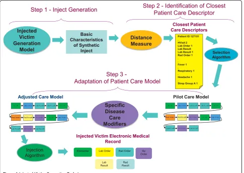
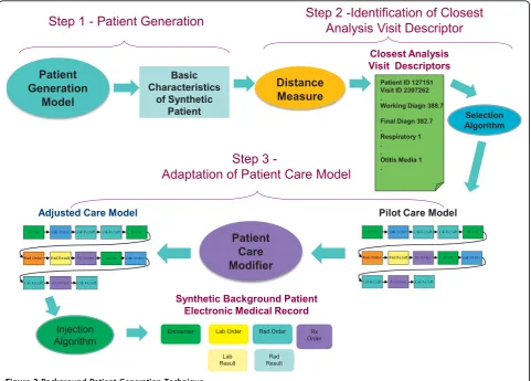
We have developed two methods, one for generating synthetic EMRs for patients included in an infectious disease outbreak (Figure 1) and the second for generat-ing synthetic EMRs for background patients (Figure 2). While these two methods share many features, there are significant differences between them. When describing

the methods below, we will point both to similarities and differences between the two techniques.

The synthesis of EMRs for either an injected disease out-break or for a set of background medical records begins with the determination of who becomes ill (or injured), when they become ill (or injured), and what diseases (or injuries) are the underlying causes of their seeking medical care. In this paper, we will refer to these simulated patients with the disease of interest as the victims. Therefore, the two techniques may be called respectively theInjected Vic-tim Generation Technique(Figure 1), and theBackground Patient Generation Technique(Figure 2).

Once the basic information about patients has been synthesized (date of birth, gender, etc.), the next step is the identification of the care patterns that the synthetic patients would receive. This care pattern is defined as the sequence of health-care events that the patient experiences and it is used to create entries in the syn-thetic EMR. These EMR entries may include laboratory test orders/results, radiology orders/results, and pre-scription orders, as well as the clinical history such as working and final diagnoses.

After an appropriate care pattern is identified from the care patterns present in the real EMR data set - the method is described in detail in [49], the creation of the full EMR for the synthetic patient can proceed. The EMR creation steps for theInjected Victim Generationdiffer somewhat from those for theBackground Patient Genera-tion. Both include the time-stamping of various parts of the EMRs so that the visit time of the synthetic patient and the timeline of the care pattern match, although with some added noise. Both include the assignment of fictitious lab test and radiology order numbers, and the subsequent renumbering of matching results occurs in both techni-ques. The synthetic background records require sanitiza-tion of clinician names, dates and addisanitiza-tional reporting events from any records and removal of details, e.g. allu-sions to specific injury scenarios on radiology results, so that the records could be meaningfully adapted to the syn-thetic patients. Compared with the background patients, the creation of the synthetic injected disease victim EMRs includes the additional step of altering the information in test and radiology results to simulate those data that would be expected for patients with the particular disease of inter-est. This step utilizes information such as disease incuba-tion period ranges, frequencies of particular presenting symptoms and signs, disease progression and severity, test results, etc., that may be found in case reports and litera-ture describing outbreaks of the injected disease.

II.b Definitions Inject

(4)

The synthetic EMRs of patients who are infected with the disease of interest will be calledinjects.

Victims

The synthetic patients who are infected with the out-break disease of interest will be calledvictims.

Background records or patients

The EMRs of patients other than those with the disease of interest will be calledbackground records.

Care Model (also called Care Pattern)

A Care Model is defined as the sequence of health-care events that a patient experiences. These care models are identified from real EMR data and described in detail in section II.e.

Rx

The abbreviationRxwill be used for prescriptions.

II.c Data Set

We developed the synthetic EMR creation techniques using a dataset that contained 14 months of EMRs from the BioSense [32] program. These data represented 458,346 patients that belonged to five age groups (0-3, 4-11, 12-19, 20-49, 50+ yrs). The records were first

anonymized by removing the patients’identifying infor-mation (e.g., name, social security number, address). To further protect patient privacy, the records were pro-cessed via the RBNR [6] algorithm to shuffle visit dates within a two-week period and patient ages within an age group. The original EMR data were from a metropolitan area in the Midwestern United States.

These BioSense data included seven tables defined as follows: 1) the Analysis Visit Table, which includes patient and visit identifier numbers, age and gender information, a summary of clinical activity, and syn-drome and sub-synsyn-drome; 2) the Clinical Activity Table, which includes patient identifiers and detailed records of chief complaint/reason for visit, working diagnoses and final diagnoses; 3) Laboratory Orders; 4) Laboratory Results; 5) Radiology Orders; 6) Radiology Results; and 7) Rx (defined as prescription) Orders. All tables for a particular patient were linked via a patient identification number and a visit identification number. The tables were in the format used by the SAS system [33].

(5)

Patient Generation. For the victims, we extracted from the full data set records of patients who had symptoms similar to those exhibited by patients with any stage of tularemia. Typically, these patients have fever and some combination of cough, chest pain, sore throat, painful respiration, malaise/fatigue, sometimes diarrhea or nau-sea and vomiting; in later stages they could have hemoptysis, respiratory failure and enlarged lymph nodes. A query on the whole data set to retrieve patients who have combinations of the symptoms described above identified a subset of over 10,000 patients. The rest of the operations for synthetic EMRs of tularemia victims were performed on that subset.

For theBackground Patient Generation, we extracted from the whole data set the patients from each of age groups: 0-3, 4-11, 12-19, 20-49, 50+ yrs. In further research we concentrated on the 4-11 age group that had 12,599 patients. All data extraction was done via SAS procedures, with most extracted frequencies and tables of data values exported to .csv (comma-separated value) or .xls (Excel spreadsheet) files. We constructed the progression of illness and created patient identities

for the injected tularemia patients, constructed the syn-thetic patient timelines and identities for the back-ground data, and wrote the synthetic EMRs for both sets of patients using Matlab functions. Most of the data analyses and comparisons were performed using Matlab [34]. The computing time necessary for these steps was minimal, on the order of a few minutes.

II.d Step One: Synthetic Patient Identity and Basic Information Generation

The first major step of our method (see Figure 1 and Figure 2) is the generation of the synthetic patient iden-tities and basic information about the synthetic patients. Because there are some differences in the method for Injected Victim Generationand the Background Patient, these will be described separately in the next two sections.

Injected Victim Record Generation (Figure 1)

(6)

disease dictates the epidemic curve, the type and sever-ity of symptoms, and the disease progression. For exam-ple, in the simulated bioterrorist release of tularemia, the release of airborne tularemia occurred in the restrooms near the luxury boxes at a summer sporting event. The timelines for the initial prodrome and then full-blown illness were taken from values in the litera-ture [35,36] that were identified for primary pneumonic tularemia. The expected symptoms, signs, and progres-sion of disease for the simulated victims were adapted from case studies and disease descriptions in the litera-ture (e.g., [36]). For the synthetic tularemia outbreak, we considered patterns of care and produced synthetic vic-tims for the entire metropolitan area and all age groups present at the sporting event (all groups except for 0-3 year olds).

The timelines and illness progression for the synthetic tularemia victims were dependent on the dose of bacter-ial particles to which each victim was exposed, age, and other disease information found in the literature [35-40]. Because the simulated exposure was to take place in the restrooms at a sports venue, the bacterial dosages for women were slightly higher than for men based on stu-dies showing that women generally spend longer in the restroom than men [41]. A small subset of the victims sought care for influenza-like prodrome symptoms from 4 to 7 days after exposure and returned with increased severity of symptoms 14 to 18 days later. Most victims sought care 18 to 22 days after exposure. We synthesized these patients with demographic information and chief complaints. Using information from literature describing the disease presentations and progression [35-37,40], we compiled a list of symptoms, signs, and their probability of occurrence in patients infected with the disease. For the 10% of the patients who sought care for the initial flu-like illness, symptoms were fever/chills (95% of patients), cough (non-productive) (38%), headache (45%), sore throat(15%), malaise/fatigue (50%), muscle aches (25%), chest pain (20%), nausea and vomiting (20%), joint pain (15%), abdominal pain (10%), and painful pink eye (5%). For severe illness, occurring 18-22 days after expo-sure, the possible symptoms were fever/chills (in 85% of patients), difficulty breathing (in 30% of patients), short-ness of breath (in 24% of patients), hemoptysis (in 11% of patients), respiratory failure (in 12% of patients), rash (30%), chest pain (40%) and cough (65%). Of the people seeking care for severe illness, 10% were chosen to have fever, abdominal pain, nausea, vomiting, and diarrhea, as these are symptoms of sepsis that are particular to tulare-mia [35].

Using the syndromes and sub-syndromes assigned to the injected patients and a distribution of additional patient attributes that we compiled from the literature, we produced a victim descriptor for each patient. The

victim descriptor included the basic characteristics of the injected patient: age, gender, race, ethnic group, cer-tain syndromes and sub-syndromes related to tularemia (described in the previous paragraph). These victim descriptors were then passed to the next step (identifica-tion of closest care models) of the EMR synthesis procedure.

It is worth noting that the real EMRs we used did not contain any diagnoses of tularemia. Thus, using expert medical opinion, we searched for patterns of care that matched the sequence of symptoms that were generated in the course of simulating the illness progression in each synthetic victim. This procedure is described in detail in section II.e. In some cases patterns of care could be found that were quite close to what was expected for tularemia and in some cases there were discrepancies; we describe the required adjustments to the data in section II.f.

Synthetic Background Records Generation (Figure 2) There is no single scenario or target population when the intention is to produce synthetic background records. The underlying causes of symptoms and rea-sons for seeking care are not known and need to be imposed on the synthetic patients in an approximation of those that appear in the real EMRs. However, the real EMR is an inexact reflection of the underlying condition of a patient. Even the most carefully entered EMR has been filtered by medical personnel subject to insurance rules and hospital or office protocols (see, e.g. [42]). To synthesize the background patients, these real EMRs must be analyzed for the probable underlying illnesses and injuries and their timelines. The pilot group of patients for the synthetic background records was the 4-11 year age group. We further restricted the patterns of care and synthetic patient demographics to a 5-county area including the metropolitan area and some sur-rounding suburban areas. We used the timelines in the clinical activity record as the data to drive creation of the synthetic patient identities.

(7)

Another, even more relevant, consideration is the defi-nition of the mapping from the driving data element to illness. By the mapping from data element to illness, we mean the identification of a single value of a data ele-ment with a particular illness, injury or condition. Ide-ally, the data element used to define the patients would have a clear and easily recognized relationship to under-lying illness or injury. The mapping from data element to illness is“well defined”in the real data if the patient visits are grouped by a single value of this data element and if it differs very little in the underlying illness or condition that can be inferred from the information in the medical record. This is akin but not equal to the notion of specificity; a well-defined mapping minimizes the inclusion of dissimilar records associated to the data element. This mapping also has to be well-defined in the inverse sense, meaning that there is littleoverlap in the underlying illness or injury (as manifested in the EMR) for patient visits that are grouped by different values of the data element. This notion is akin but not equal to sensitivity; a well-defined inverse mapping minimizes the number of data elements that are asso-ciated with similar electronic medical records. If such a mapping is reasonably well-defined in both directions, the timelines of different values for this data element could be mimicked to impose the entire spectrum of ill-ness and injury to a synthetic population via an auto-mated process. If the mapping is not well-defined, using this data element to drive the synthetic population

creates several problems. We illustrate the possible pro-blems by considering the mapping for various candidate data elements in the EMR.

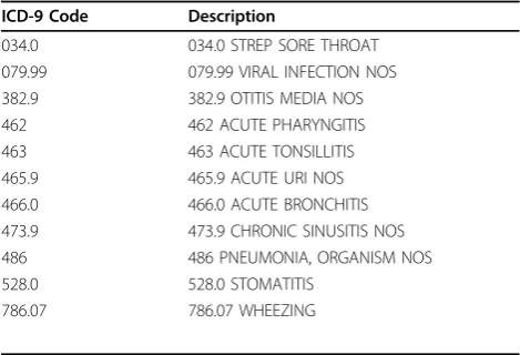
First let us consider the use of chief complaint, syn-drome or sub-synsyn-drome as the driving data element. Because of the variations in the spelling and abbrevia-tions in chief complaints, the additional step of natural language processing (e.g. [44,53]) is necessary to cate-gorize chief complaints in advance of associating them with particular illnesses. Even with the use of a natural language processor, this association is not particularly well-defined. For example, the chief complaint sore throat(and many variations) appears quite often in this age group. However, sore throat can define or be pre-sent in multiple illnesses. Table 1 shows the diagnoses that are extracted from the real data for the chief com-plaint sore throatfor this age group. Similarly, the 10 syndrome definitions and 68 sub-syndrome definitions do not exactly define an illness or injury. Although mul-tiple chief complaints, syndrome definitions and sub-syndrome definitions can more accurately describe the illness or injury, this mapping is still inexact.

There are different possible illnesses or injuries that may be associated with a chief complaint, syndrome or sub-syndrome and the inverse is also true: there are many possible chief complaints for each underlying ill-ness (or injury). To illustrate this, we extracted all patient visits with a single final diagnosis code of strep throat (ICD-9 code 034.0) from both emergency and outpatient cases in the subset of 4-11 year old patients from the real data set. Among emergency cases, there were 49 different chief complaint strings, taken from a list of 28 different single complaints (e.g. fever, nausea, neck pain, cold, cough, stuffy nose, abdominal pain, vomiting, sore throat or variations such as throat pain, throat sore, etc. as well as others). Although sore throat (and variations) appeared quite often in the strings, there were 26 complaints (53%) that did not contain sore throat, throat pain, or other such variations any-where in the complaint text. In the outpatient cases, there were 62 different reasons-for-visit, with 30 differ-ent single complaints. Of these, 9 (14.5%) did not con-tain sore throat, throat pain or other such variations anywhere in the reason-for-visit text. This ill-defined mapping translates to the following problem with using chief complaint as the driving data element. If patients were synthesized only from timelines of particular chief complaints, the variety of underlying causes would have to be synthesized independent from, but consistent with, the chief complaints. This would require either consid-erable expert input on the possible conditions associated with those chief complaints or the categorization of ICD-9 codes and/or syndromes and sub-syndromes by chief complaint.

Table 1 Data elements present in the real data set

Data Element % of visits in model data

Chief Complaint or Reason for Visit 85.16

Sub-syndrome 83.52

Syndrome 54.41

Final diagnosis ICD-9 code 99.72

Table 2 Possible ICD-9 codes associated with the chief complaint“sore throat”

ICD-9 Code Description

034.0 034.0 STREP SORE THROAT

079.99 079.99 VIRAL INFECTION NOS

382.9 382.9 OTITIS MEDIA NOS

462 462 ACUTE PHARYNGITIS

463 463 ACUTE TONSILLITIS

465.9 465.9 ACUTE URI NOS

466.0 466.0 ACUTE BRONCHITIS

473.9 473.9 CHRONIC SINUSITIS NOS

486 486 PNEUMONIA, ORGANISM NOS

528.0 528.0 STOMATITIS

786.07 786.07 WHEEZING

(8)

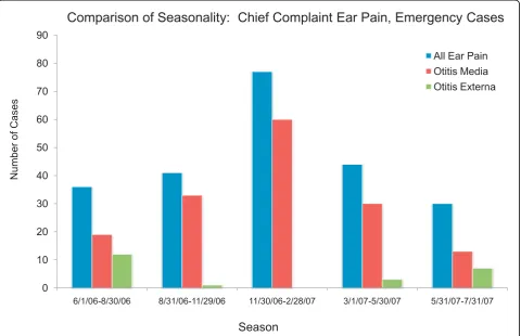
An additional difficulty with using chief complaints, syndromes or sub-syndromes is that temporal variations in specific conditions would be inherited from the gen-eral category of data elements and may not match those for specific illnesses in the real data. For example, ear pain may be associated with Otitis externa or Otitis media. Otitis externa exhibits different seasonal inci-dence from otitis media (see Figure 3) but, if chief com-plaint were used to drive the synthetic patient data, neither seasonal variation would be apparent. The inverse mapping from illness to chief complaint is also important for this reason. If cases for a particular illness (e.g. strep throat - see Figure 4) are spread across more than one chief complaint (as they usually are), it is diffi-cult to recover the timeline for this illness reliably from the chief complaints. Conversely, different timelines for variations in a syndrome or subsyndrome (e.g. falls) can-not be recovered by using the timeline for the syndrome or sub-syndrome alone (see Figure 5).

Next, let us consider using ICD-9 code as the driving data element. Although the final diagnosis ICD-9 code does not always completely describe or define the underlying illness or injury of a patient [45,46], there is

a relatively clear relationship between final diagnosis ICD-9 code and the care that a patient would receive, as well as possible chief complaints, syndromes and sub-syndromes. There is some overlap in the mapping from underlying illness or injury to ICD-9 code, because of inexact coding, coding conventions and insurance reim-bursement rules. The timelines for specific ICD-9 codes should reflect, to a certain degree, seasonal or sporadic variations in disease and injury occurrences. We also note that this is the data element that is least likely to be omitted in an EMR. Thus, we settled on the final diagnosis ICD-9 code as the “driving” data element. In other words, we replicated statistical and mathematical properties of the ICD-9 code time series and used those to impose those illnesses and injuries on the synthetic patients. All attributes of the patients were chosen by using the final diagnosis ICD-9 code as the determining variable for age (within the age group), gender, race/eth-nic group, and syndrome and sub-syndrome classifica-tions. The use of a single ICD-9 code as the driving data element proved to be sufficient for this age group because the majority of the visits in the real data exhib-ited a single ICD-9 code. Other age groups may require

(9)

a multi-dimensional ICD-9 code map, depending on the characteristics present in the real data.

The BioSense dataset contained 6426 clinical activity records for Emergency (ER) patients and 3248 records for outpatient (OP) patients. Of the 6426 ER visit records, 65% of the visits had 29 different final diagnosis ICD-9 codes with 100 or more patient visits. These 29 included ICD-9 codes 873., 382., 493., 465., and 034 as the codes with the most patient visits; those 5 ICD-9

codes comprised 28% of the patient visit records. How-ever, we reconstructed timelines for 295 ICD-9 final diagnosis codes for the synthetic ER patients. Of the 3248 OP visits, 43% of the visits had 14 different final diagnosis ICD-9 codes with 60 or more patient visits. These 14 included codes 382, 079, 462, and 034.

Because the primary diagnosis and any secondary diagnoses were not differentiated in the BioSense dataset we received, we used a convention to define the primary Figure 4The inverse map from underlying illness to Chief Complaint is not well defined; multiple overlapping and non overlapping chief complaints contain the strep throat cases.

(10)

diagnosis. For each patient in the real data set, we sorted the final diagnosis codes in numeric order, with the exception that specific injury codes (prefixed E) were excluded from occurring as primary diagnoses. The first code (after alphanumerically sorting) was defined to be the primary diagnosis. The time series of healthcare events related to this primary diagnosis were mimicked to produce the synthetic patient timelines. Furthermore, we verified that this set of primary diagno-sis ICD-9 codes did not contain diagnoses that were either considered rare by a subject matter expert or never appeared as a single primary diagnosis. This pro-cedure thereby assured that sorting the ICD-9 codes and using the first code as the primary diagnosis did not omit any other potential primary diagnoses.

Rare diagnoses, diagnoses that are unusual in this age group, and diagnoses that included multiple congenital conditions were excluded from consideration because an individual could be identified from such a diagnosis together with knowledge of the particular region. Produ-cing multiple records from these ICD-9 codes in order to remove the possibility of identification would yield a higher-than-usual incidence of rare or unusual conditions in the synthetic data. Although it could be argued that exclusion of rare diagnoses reduces the fidelity and realism of the synthetic data, a data set without theparticularrare diagnoses that were excluded is not unrealistic. Care mod-els for randomly chosen rare or unusual illnesses or condi-tions could be synthesized using expert opinion to improve the realism of a large synthetic data set.

We extracted the timelines of truncated (without detail codes after the decimal point) final diagnosis ICD-9 codes from the clinical activity records of the real data and reconstructed similar (but not identical) timelines in two ways, dependent on the sparseness or richness of the data stream. For time series with on average more than 1 case per week, we performed a Haar wavelet-2 [47] reconstruction to de-noise but replicate the fre-quencies in the time series. We tested reconstructions using both Haar and Daubechies wavelets as well as a reconstruction based on nonlinear prediction (see, e.g. [48] section 4.2). The Haar wavelet-2 reconstruction yielded the best prediction in terms of root-mean-square (rms) values and total numbers of cases. For time series with less than 1 case per week, we calculated seasonally-varying weekly Poisson parameters. We reconstructed those time series by taking Poisson draws from the spe-cified distribution, and by using day-of-week probabil-ities from the actual time series (again, adjusted seasonally) to assign a day of the week to the cases. Demographic data was extracted from the real data, keyed from primary final diagnosis ICD-9 code, and assigned to each synthetic patient based on the primary ICD-9 code. The birth date for each synthetic patient

was chosen randomly based on the synthetic patient’s age to further distance each synthetic patient’s identity from that of a real patient. Additional ICD-9 codes were assigned to the synthetic patients according to a season-ally varying multivariate distribution dependent on pri-mary diagnosis ICD-9 code. Sub-syndromes and syndromes were assigned to the synthetic patients dependent on all the final diagnosis ICD-9 codes using the patterns extracted from the real EMR data. The patient’s visit descriptor with the basic characteristics of the synthetic patient’s visit includes patient’s age, gen-der, race, ethnic group, syndromes, sub-syndromes, and final diagnosis ICD-9 codes. At this point, the basic visit descriptors for the synthetic patients contained enough information for the identification of closest patient care descriptors (Figure 2) to proceed. We note that the chief complaint is that of the pattern of care rather than chosen from a distribution based on the final diagnosis ICD-9 code. Since the synthetic background patients were created from ICD-9 code streams of the real patient population, the patterns of care that this popula-tion would receive were present in the real data. We note that the synthetic patients mimicked rather than exactly duplicated the real patient population: no syn-thetic patient matched a real patient exactly in age, gen-der, demographic variables and visit information (ICD-9 codes, syndromes and sub-syndromes) although as a group the age, gender, demographic variables and ICD-9 diagnoses displayed the same statistical distributions as the real data. Although this was precisely the intent of producing completely synthetic patient identities, this inexact matching made locating appropriate patterns of care for the synthetic patients complicated. This method cannot match the multidimensional data fidelity of, for example, a shuffling and anonymization algorithm (e.g. RBNR). However, it does reproduce many of the multi-ple dimensions present in the real data (see verification results here and in [49]) and mitigates many objections to dissemination of anonymized and shuffled data. In the next section we describe, in detail, the methods for identifying patterns of care for both the injected disease victims and for the background synthetic patients. The identification of the pattern of care for the background patients is another safeguard for anonymization. Although it was not necessary for this particular data set, the algorithm that chooses the care model can be adapted to exclude any exact matches in demographics, ICD-9 codes, syndromes and sub-syndromes from consideration.

II.e Step Two: Identification of Closest Patient Care Models and Descriptors

(11)

characteristics of the synthetic patient are coming from the Injected Victim Generation Model (see Figure 1)/ Background Patient Generation Model(see Figure 2). They include syndromes, sub-syndromes, age, gender, race and ethnic group of each synthetic patient. For the background patient EMRs, these characteristics addi-tionally include visit information and the final diagnosis ICD-9 codes.

Step 2 for Injected Victim Generation operates on Patient Care Descriptors (Figure 1) and for Background Patient Generationit operates onAnalysis Visit Descrip-tors (Figure 2). A distance measure is defined, and the closestPatient Care Descriptor/Analysis Visit Descriptor is identified in the original data set. The information from thisPatient Care Descriptor/Analysis Visit Descrip-tor is next given to major step 3:Adaptation of Patient Care Model. The steps mentioned need to be executed separately for each synthetic patient (and for each visit in case of Background Patient Generation. These steps are described in detail in Section II.f.

Before the above steps can be executed, Patient Care Models, Patient Care Descriptors, and Analysis Visit Descriptors need to be extracted from the EMR data set. This is a process that is performed only once for the whole data set. It is described in detail later in this section. The computation of Patient Care Models and Patient Care descriptors is computationally expensive: it takes about 30 sec per patient. For 10,000 patients such a computation takes about 80 hours on a 32-bit PC. Patient Care Models

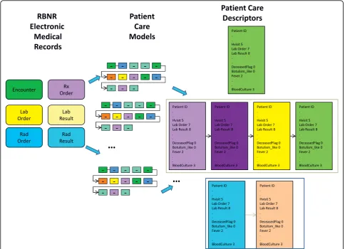
APatient Care Model[50] is a sequence of all the health care encounters (that we will also call events) that were present in the original EMR data set for a given patient. The care model consists of up to seven types of events: 1) Analysis visit (abbreviated AVisit); 2) Laboratory order; 3) Laboratory result; 4) Radiology order; 5) Radiology result, 6) Prescription order (abbreviated Rx), 7) Death event - if applicable. The events in the extracted care model are sequentially ordered based on the dates and times they occurred (as present in the data).

The AVisit contains the information about a given patient visit including patient’s demographic data, visit identification number, visit date, syndromes, and sub-syndromes. For Background Patient Generation, AVisit also incorporates working diagnoses ICD-9 codes and final diagnoses ICD-9 codes. The demographic data con-sists of patient birth date, age, race, ethnic group, and gender. Inside the laboratory orders, there is information on each of the laboratory tests that were ordered during a given visit, including date and time. In the laboratory results, there is information on each of the labs with, for example, bacteria identified or information that the test was negative. Individual Patient Care Models are of dif-ferent lengths (depending on the number of visits and

specific information in laboratory orders, laboratory results, radiology orders, radiology results and Rx orders). People who came only once and did not have any laboratory or radiology orders have patient care models with one record. People who came many times and had many laboratory or radiology orders and results have very lengthy care models (hundreds of records). Figure 6 shows the Patient Care Model for a 4-11 year old girl with two AVisits, one laboratory test (for Strep), one radiology test (DX Sinus paranasal complete) and one radiology result (DX Sinus paranasal complete). Patient Care Descriptors

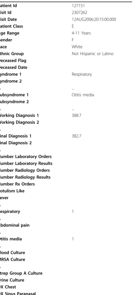
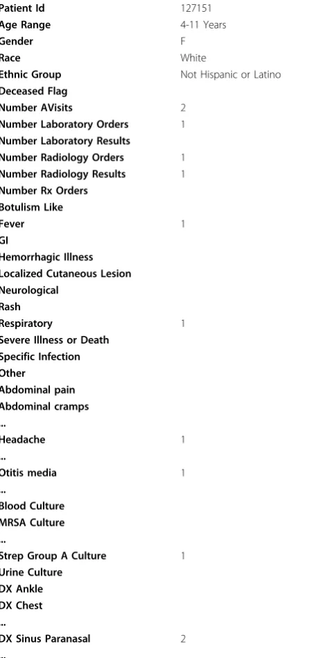
Patient Care Descriptorssummarize Patient Care Mod-els. For each Patient Care Model, one Patient Care Descriptor is computed. ForBackground Patient Gen-eration, Patient Care Descriptors consist of individual Analysis Visit Descriptors(see Table 3 and Table 4) that describe a given visit in detail, including any laboratory and radiology tests related to that visit. The Analysis Visit Descriptor for visit 2307262 is shown in Table 3. It has many empty fields because there were no laboratory or radiology orders or results related to that visit. The Analysis Visit Descriptor for visit 3102841 (Table 4) is more complicated because it contains information on one laboratory order, one radiology order and one radi-ology result. If a given patient (e.g., the one from Figure 3) had two visits, his or her Patient Care Descriptor will consist of two Analysis Visit Descriptors chronologically ordered. For that patient, the Patient Care Descriptor encompasses the Analysis Visit Descriptor for visit 2307262 and the Analysis Visit Descriptor for visit 3102841. Should the patient visit the hospital often and have 30 analysis visits, his or her Patient Care Descrip-tor would consist of 30 Analysis Visit DescripDescrip-tors.

ForInjected Victim Generation because lower level of detail was available, Patient Care Descriptors summarize all the care given to a patient without distinguishing for which Avisit the care occurred. An example Patient Care Descriptor forBackground Patient Generation is shown in Table 5. In addition to patient identification number, ethnic and demographic information, it con-tains the numbers of AVisits, laboratory orders and results, radiology orders and results, Rx orders, all the syndromes, sub-syndromes, types of laboratory and radi-ology tests, and test results.

Extraction of Existing Patient Care Models and Descriptors The goal of the methodology developed is to derive, from the available real EMR data, a care model of how the patients are treated. This method has the following main steps (Figures 7 and 8):

1) Build Patient Care Models - sequences of patient care events for each patient.

(12)

Figure 7 shows the procedure for Injected Victim Generation, and Figure 8 shows the procedure for Back-ground Patient Generation. The first part of the proce-dure is exactly the same in both cases: Patient Care Models are computed from the EMRs anonymized by the RBNR algorithm and; all seven tables (described in Section II.c) with RBNR records are accessed in order to extract all the information pertaining to a given patient.

For Synthetic Inject Records Generation (Figure 7), the Patient Care Descriptors are determined next, one descriptor per patient. An example Patient Care Descriptor was shown in Table 5. However, for Back-ground Patient Generation (Figure 8), the procedure is slightly more complicated: after the calculation of Ana-lysis Visit Descriptors (one descriptor per anaAna-lysis visit), they are grouped into Patient Care Descriptors. The Analysis Visit Descriptors are ordered by occurrence date in the Patient Care Descriptors. The process of building both Analysis Visit and Patient Care descriptors is completely data driven: if there arendifferent micro-organisms identified in the data set, there will be n

corresponding fields in the descriptor; if there arem dif-ferent types of laboratory tests in the data set, there will bemcorresponding attributes in the descriptor.

Identification of Closest Descriptors

The information coming from Step One into Step Two is different for the Injected Victim Generation (Figure 1) and Background Patient Generation (Figure 2). For Injected Victim Generation, this information does not include any data about individual visits for a given patient (Figure 1). For our tularemia example, this infor-mation only contains certain syndromes and sub-syn-dromes related to tularemia-like illness at different stages of disease progression (e.g., fever, cough, head-ache, sore throat, malaise and fatigue, muscle aches, chest pain, nausea and vomiting, abdominal pain, diffi-culty breathing, respiratory failure, rash). This is the rea-son for having the matching algorithm, subsequently described, operate on Patient Care Descriptors.

(13)

patient visit including syndromes, sub-syndromes, and final ICD-9 codes (Figure 2). Because of the high granu-larity of this information, it is possible to operate on individual patient visits, and hence the matching algo-rithm uses Analysis Visit Descriptors.

ForInjected Victim Generation, the process of finding the closest set of patient care descriptors is shown as

step 2 on Figure 1. A distance measure is computed between the inject descriptors and existing Patient Care Descriptors. The few closest descriptors are identified (Distance Measure). Next, the patient care models corre-sponding to the Closest Patient Care Descriptors are selected from the background data (Closest Care Model).

Table 3 Example Analysis Visit Descriptor (for Visit 2307262)

Patient Id 127151

Visit Id 2307262

Visit Date 12AUG2006:20:15:00.000

Patient Class E

Age Range 4-11 Years

Gender F

Race White

Ethnic Group Not Hispanic or Latino

Deceased Flag Deceased Date

Syndrome 1 Respiratory

Syndrome 2

... ...

Subsyndrome 1 Otitis media

Subsyndrome 2

... ...

Working Diagnosis 1 388.7

Working Diagnosis 2 ...

Final Diagnosis 1 382.7

Final Diagnosis 2 ...

Number Laboratory Orders Number Laboratory Results Number Radiology Orders Number Radiology Results Number Rx Orders Botulism Like Fever ...

Respiratory 1

...

Abdominal pain ...

Otitis media 1

...

Blood Culture MRSA Culture ...

Strep Group A Culture Urine Culture DX Chest

DX Sinus Paranasal

Table 4 Example Analysis Visit Descriptor (for Visit 3102841)

Patient Id 127151

Visit Id 3102841

Visit Date 10JAN2007:08:41:07.000

Patient Class E

Gender F

Race White

Deceased Flag Deceased Date

Syndrome 1 Fever

Syndrome 2 Respiratory

... ...

Subsyndrome 1 Fever

Subsyndrome 2 Headache

... ...

Working Diagnosis 1 462

Working Diagnosis 2 ...

Final Diagnosis 1 462

Final Diagnosis 2 465.9

...

Number Laboratory Orders 1

Number Laboratory Results

Number Radiology Orders 1

Number Radiology Results 1

Number Rx Orders Botulism Like

Fever 1

...

Respiratory 1

...

Abdominal pain Abdominal cramps ...

Headache 1

...

Strep Group A Culture 1

Urine Culture DX Chest

(14)

A distance measure is used to identify the closest (minimum distance) Patient Care Descriptor to the desired inject. Gower’s General Similarity Coefficient [51] and several Euclidean distances were investigated. The distance measure needs to be well-tuned to the ill-ness of interest because its goal is to identify the patients who have attributes similar to those of the inject. Certain attributes are not related to tularemia, and therefore their presence or absence is inconsequen-tial and for that reason these attributes will not be used

in the distance measure. An example of such an attri-bute is Cardiac dysrhythmiasbecause whether or not a person has Cardiac dysrhythmiassub-syndrome, this person may have symptoms similar to those of tularemia and the treatment will also be similar.

The Euclidean distance operates on the following 23 attributes: Syndrome attributes - Fever, Gastrointestinal, Rash, Respiratory; and Subsyndrome attributes -Abdominal pain, Alteration of consciousness, Chest pain, Convulsions, Cough, Diarrhea, Dyspnea, Headache, Hemoptysis, Hemorrhage, Influenza-like illness, Lym-phadenopathy, Neoplasms, Malaise and fatigue, Nausea and vomiting, Respiratory failure, Septicemia and bacter-emia, Upper respiratory infections, Severe illness or death.

The Euclidean distance, dist(I, P), between the inject descriptor I, and existing Patient Care Descriptor P is defined as:

dist I P

(

,

)

= Σ_i23₌₁w_i

(

I_i−P_i

)

2 (1)

Where wi = 1 for 1≤=i≤= 22, andw23= 0.1; Iiand

Pisignify the value of a given attribute (from the

attri-butes specified in the previous paragraph) for the inject descriptor and patient care descriptor, respectively. The attribute for which the weight of 0.1 is used isSevere ill-ness or death. One might ask why one of the attributes used in the distance measure is neoplasms: neoplasms have nothing to do with tularemia, so why use this sub-syndrome in the distance measure? The fact that they have nothing to do with tularemia is precisely why they are needed. Before we included neoplasms in the dis-tance measure, most of the closest patient care descrip-tors retrieved for injects with malaise and fatigue had neoplasms. We wanted to exclude patients with neo-plasms because their care models are too different from those with tularemia. Therefore, for all the injects, we set the neoplasms attribute to 0, and using the distance measure in Eq. (1), we were able to retrieve patient care descriptors that had no neoplasms as diagnosis. Ten nearest neighbors (in terms of the Euclidean distance), from the same age group as the inject are retrieved. These nearest neighbors are processed by theSpecific Disease Care Modifier(described in Section II.f).

For the Background Patient Generation, the procedure described below is performed for every synthetic visit of every synthetic patient. The goal is to find, for each syn-thetic visit, a visit that is as similar as possible in the real data. Figure 9 depicts how the closest analysis visit descriptor to a synthetic visit descriptor is determined. The basic characteristics of the synthetic patient, in the form of information about synthetic visits for a given patient, are produced byPatient Generation Model(see

Table 5 Patient Care Descriptor for Patient 127151

Patient Id 127151

Gender F

Race White

Deceased Flag

Number AVisits 2

Number Laboratory Orders 1

Number Laboratory Results

Number Radiology Orders 1

Number Radiology Results 1

Number Rx Orders Botulism Like

Fever 1

GI

Hemorrhagic Illness Localized Cutaneous Lesion Neurological

Rash

Respiratory 1

Severe Illness or Death Specific Infection Other

Abdominal pain Abdominal cramps ...

Headache 1

...

Otitis media 1

...

Strep Group A Culture 1

Urine Culture DX Ankle DX Chest ...

DX Sinus Paranasal 2

(15)

Figure 2). Each synthetic visit is characterized by final diagnosis ICD-9 codes, syndromes, sub-syndromes, age, gender, race and ethnic group of the synthetic patient. A distance (the distance measure used is described further in this section) is computed between a given synthetic visit and all the analysis visit descriptors resulting in a set of closest (i.e. minimum distance) ana-lysis visit descriptors. All the information about that visit is extracted from the corresponding Patient Care Model.

We define a distance measure between a synthetic visit and an Analysis Visit Descriptor that is a combina-tion of weighted Euclidean distance and Jaccard distance [52]. The Jaccard index (or similarity coefficient) mea-sures similarity between two sets, and is defined as the size of the intersection divided by the size of the union of the sets:

J A B A B A B

( , )= ∩

∪ (2)

The Jaccard index is a useful measure of similarity in cases of sets with binary attributes because it takes into account not only how many attributes agree but also how many disagree. If two sets, A and B, haven attri-butes each, then Jaccard index measures the attribute overlap that A and B share. The Jaccard distance is then defined as:

J A B J A B A B A B

A B

dist( , )= − ( , )=

∪ − ∩

∪

1 (3)

We defined and used the following distance measure to identify the closest Analysis Visit Descriptor to a given synthetic visit descriptor:

dist A S( , )=J_dist( , )A S + Edist( , )A S

70 (4)

where Astands for Analysis Visit Descriptor,S - for Synthetic Visit Descriptor, andEdist- for Euclidean

(16)

attributes: truncated final diagnosis ICD-9 codes, syn-dromes, and sub-syndromes; Euclidean distance is only computed on a non-binary attribute (age). Jdist(A,S) has

a value between 0 and 1 (inclusive) and Edist(A,S) has a

value between 0 and 7 (inclusive). In order to make both distances contribute the same to the final distance measure, Edist(A,S) would have to be divided by 7.

When designing dist(A,S) we wanted the age attribute to contribute only 1/10 as much as the Jdist(A,S).

There-fore, we need to divide the Euclidean distance by 70 in Equation 4 above. Because it is most important to have agreement on as many final diagnosis ICD-9 codes, syn-dromes, and sub-syndromes as possible, the agreement in age between Analysis Visit Descriptor and Synthetic Visit Descriptor is secondary.

Next we examine the search methods and rationale behind assignment of a specific care model to a syn-thetic patient. These processes differed both in automa-tion level and in specific procedures for the synthetic tularemia victims and for the synthetic background patients.

II.f Step Three: Adaptation of Patient Care Model Care Model Assignment and Adaptation

The third step in the process (see Figure 1 and Figure 2) is adapting the chosen care model to the specific syn-thetic patient and actually writing the electronic medical records. During the development of this project, the methodology evolved significantly between the creation of the injected tularemia victims and the creation of the synthetic background records. We were able to auto-mate nearly all of the steps for adaptation of care mod-els for the synthetic background patients but there was considerable non-automated effort in the adaptation of the care models for the synthetic tularemia victims.

(17)

If respiratory or blood cultures were taken, we modified results to indicate no growth, reflecting the fastidious nature of tularemia in routine cultures. In some cases, we added chest x-rays to the records of patients whose care models did not include them to suggest a physi-cian’s possible response to an unexplained severity or persistence of respiratory symptoms. Chest x-ray results were modified to include evidence of pathology that would be common for pneumonic tularemia patients. Because the care models had to be inspected and edited individually and the patients assessed based on the symptoms generated by the injection algorithm, little automation was possible for this phase of the synthetic tularemia injection method. This is the biggest drawback of the methodology proposed.

In the case of Background Patient Generation, the dis-tance measure used to find care models identified up to ten care model candidates for each synthetic back-ground patient. We automated the process of choosing the most appropriate care model from those identified by examining specific ICD-9 codes and exact syndromes and sub-syndromes in the patient visit records and in the care models. The hierarchy was first to try to match

all exact ICD-9 final diagnosis codes in the patient visit record. If multiple care models still matched the patient visit record, the algorithm chose by specific sub-syn-drome and synsub-syn-drome codes. If multiple care models still matched after this step, a care model was chosen ran-domly from the remaining candidates, with equal prob-ability given to each.

The final part of Step Three of the methodology is the adaptation of the entire EMR to the particular patient to assure that there is no exact match between a synthetic and a real patient. This procedure is described in the next section.

Injection Algorithm

(18)

randomly chosen (uniform) variation. Any radiology or laboratory orders are assigned unique identification numbers, and these numbers are carried through to the radiology and laboratory results if present. The algo-rithm also produces summaries of clinical activity and sub-syndrome/syndrome information in the format found in the model data and writes these in the analysis visit record. All formats found in the original records are duplicated by the injection algorithm. However, patient zip code, health department identifier, and loca-tion are not synthesized for the synthetic background records. The algorithm writes the tables to comma-sepa-rated-value (csv) files, preserving leading zeros on ICD-9 codes and producing SAS date formats as well as MS-EXCEL-readable formats.

III. Results

III.a Tularemia Injects

The simulated tularemia outbreak resulted in 203 syn-thetic victims. Of these victims, 19 individuals sought care for prodrome symptoms but none of these syn-thetic patients were admitted to a hospital at that time. All 203 victims sought care for a severe respiratory ill-ness after 18-22 days; there were 57 synthetic patient admissions and 17 synthetic victim deaths.

As part of the validation process, a medical expert reviewed all the synthetic records and determined that 42 records (i.e. 19% of the inject records) had content problems or inconsistencies. The predominant problem was a string of ICD-9 codes that did not match any of the expected symptoms of tularemia. For example, a patient would be assigned ICD-9 codes of“250.00 DMII WO CMP NT ST UNCNTR”, “272.4 HYPERLIPIDE-MIA NEC/NOS”, “410.71 SUBENDO INFARCT, INITIAL”as well as the ICD-9 code of“486 PNEUMO-NIA, NOS.” Because no cases of tularemia were found in the real data, it was expected that some difficulty would arise with matching the synthetic patient descrip-tors to an appropriate care model. Of the 221 visit records (for 203 patients), 36 were deemed unsuitable for this reason. Other problems included incompatible ICD-9 codes (2 records), for example, both “786.50 CHEST PAIN NOS”and “786.52 PAINFUL RESPIRA-TION,” exact duplication of real EMR information (2 records), and odd or incorrect ICD-9 codes (2 records) such as a diagnosis of “263.9 PROTEIN-CAL MAL-NUTR NOS.”These 42 records were adjusted manually by editing the fields that were deemed inconsistent, odd, or erroneous. It was noted by the medical expert that the presentation of tularemia in the remaining synthetic records was as expected.

The synthesized electronic medical records included syndrome and sub-syndrome classifications for the injected patients. The severe respiratory illness imposed

on the victims was manifested in EMRs that included multiple syndrome and sub-syndrome classifications. Of the 221 visits for 203 victims, over 92% exhibited the fever syndrome, nearly 80% exhibited the respiratory syndrome, and 12% had severe illness or death. There were also over 10% of patients with hemorrhagic illness and over 12% with gastrointestinal syndrome. Sub-syn-drome classifications for the injected patients included over 44% with cough, nearly 40% with dyspnea, over 47% with fever, and 19% with pneumonia or lung abscess. Many of the age 50+ patients also exhibited car-diac dysrhythmias and mental disorders. There were also more than 12% with respiratory failure and nearly 10% with shock (see Table 5 for syndromes and Table 6 for sub-syndromes).

Of the 203 patients, 107 had from 1 to 28 laboratory orders. The most common test was a blood culture, for nearly 40% of the laboratory tests. The next most com-mon test was respiratory culture and smear at nearly 13% of the tests (see Table 7). There were also some very specific tests for C. difficile toxin (11.33%) and Strep Group A (2.63%). Laboratory results were forced to be negative because of the fastidious nature of tulare-mia [37]; any bacterial cultures were forced to either exhibit the results“no growth” or normal flora.

Of the 112 synthetic patients who had radiology orders, over 80% had chest x-rays (see Table 8). Radiol-ogy results were imposed on the synthetic victims to indicate evidence of bilateral peribronchial infiltrates and multi-lobar opacities, bilateral pleural effusions, bilateral sub-segmental infiltrates with foci of peribron-chial consolidation, or miliary patterns of multiple ace-nodular opacities 3-6 mm in diameter, all characteristic of primary pneumonic tularemia (see Table 9).

For illustrative purposes, we will now follow two of the synthetic tularemia patients through the various records of the EMR, as seen in Table 10. The first patient, patient ID 214973, analysis visit ID 536919, sought care for prodrome symptoms. We see an analysis

Table 6 Syndromes assigned to synthetic tularemia injects

Syndrome % of 221 visits with listed syndrome

Fever 92.76

Gastrointestinal 12.22

Hemorrhagic Illness 10.86 Localized Cutaneous Lesion .45

Lymphadenitis 1.81

Neurological 12.67

Rash 4.52

Respiratory 79.64

Severe Illness or Death 11.76

(19)

visit date of Aug 3 2006, at which the patient reported fever and other flu-like symptoms. The syndromes assigned were fever and respiratory, and the sub-syndromes were fever and influenza-like illness. This

patient had one clinical activity record for the chief complaint, no laboratory or radiology orders (or results) and was discharged the same day. The second synthetic tularemia patient, patient ID 210042, analysis visit ID

Table 7 Sub-syndromes assigned to synthetic tularemia injects

Sub-Syndrome % of 221 visits with listed Sub-Syndrome

Abdominal Pain 8.14 Heart disease, ischemic 2.26

Alteration of Consciousness 12.67 Hempotysis 7.24

Anemia 10.86 Hypotension 1.81

Asthma 3.62 Influenza-like Illness 8.14

Bronchitis and Bronchiolitis 11.31 Intestinal infections,

ill-defined

.45

Cardiac dysrythmias 14.48 Lymphadenopathy 1.81

Chest pain 9.95 Malaise and fatigue .45

Coagulation defects .45 Mental disorders 10.86

Coma 8.14 Migraine .45

COPD 1.36 Nausea and vomiting 9.95

Cough 44.34 Pleurisy .45

Cyanosis and hypoxemia 2.71 Pneumonia and lung abscess 19.00

Death .45 Pupurae and petechiae 1.36

Dehydration 1.81 Rash 10.41

Diabetes mellitus 1.81 Respiratory failure 12.67

Diarrhea 8.60 Septicemia and bacteremia 4.52

Dizziness .45 Shock 9.95

Dyspnea 39.82 Skin infection .45

Edema 2.71 Syncope and collapse .45

Fever 47.51 Upper respiratory infections 2.26

Gastrointestinal hemorrhage

2.71 Urinary tract infections 1.81

Headache .90 Viral infection, unspecified 11.31

Table 8 Laboratory Tests for Synthetic Tularemia Injects

Ordered Test Name Local (Laboratory Test)

Percent of Tests Ordered

Ordered Test Name Local (Laboratory Test)

ASO Titer(ASO) .66 Influenza Antigen(FLUAG) 3.45

Aerobic .16 Legionella Ag Urine Culture(LEGEIA) .82

Blood Culture (BLC) 39.90 Lyme IgG .66

Blood Culture Isolator(BLDC) .66 Mono Test (MONO) .16

C Difficile Toxin A 11.33 Ova and Parasite Exam (OVAP) 2.46

C Reactive Protein (CRP) 3.28 Prealbumin (PAB) 1.64

CMV AB IgG (CMVGAB) .66 Reproductive Culture .66

CMV AB IgM(CMVMAB) .66 Respiratory Culture and Smear(RTCS) 12.97

Chlamydia/GC by Amplified .66 Respiratory Viral Panel Acute(RVPA) .66

Probe(CGPT)

Enteric Pathogen Culture(ENPC) 2.46 Strep Group A Screen Rapid(RSTREP) 2.63

Epstein Barr Virus Antibody .66 Urine Culture (URC) 10.67

Screen (EBVSRN)

Gram Smear (GRAS) .16 Urine Culture and Smear (URCS) .16

Haptoglobin (HAPT) 1.15

Herpes Virus Six Culture(HHV6Q) .66

(20)

536120, was an outpatient. This patient had a reason for visit ofcoug (sic) and fever and was assigned syndromes of respiratory and fever, sub-syndromes of cough and fever. This patient had four clinical activity records: for chief complaint, working diagnosis and final diagnosis. The patient had one radiology order and three radiology results records. This synthetic patient had a routine discharge.

III.b. Background Patient Generation

We generated approximately 3000 synthetic background patient EMRs for the 4-11 year age-group. These were generated several times to insure that the algorithms performed consistently. There were 295 different pri-mary diagnosis ICD-9 codes for the group of synthetic emergency patients and 294 different primary diagnosis ICD-9 codes for the group of synthetic outpatients.

These ICD-9 codes included both illness and injury. In fact, the most common primary diagnosis for the emer-gency room patients in this age group was head lacera-tion. To illustrate, we will follow the two synthetic background patient EMRs described in Table 11. The first (Patient ID 60343) is a 4-year old girl with chief complaint of sore throat. The synthetic patient record has a syndrome assignment of respiratory and sub-syn-drome assignment of upper respiratory infections. The clinical activity record has 3 entries - for chief com-plaint, working diagnosis of pharyngitis, and final diag-nosis of pharyngitis. There is one laboratory order and it is for a rapid strep test. There are no laboratory results for rapid strep tests in any of the synthetic EMRs, reflecting the pattern found in the real EMRs. There are no radiology orders or results for this syn-thetic patient, who had a routine discharge.

The second synthetic patient is an 11-year old boy with a chief complaint of clavicular pain. The analysis visit record has sub-syndromes of falls and fractures and dislocation. There are 4 clinical activity records: for

chief complaint, working diagnosis (chest pain) and final diagnosis (closed clavicle fracture and fall from play-ground equipment). This synthetic patient record has one radiology order, for a clavicle x-ray, and 2 radiology results, reflecting the diagnosis of clavicle fracture. This synthetic patient had a routine discharge.

The descriptors for the synthetic background patients were built from the truncated 3 or 4- digit ICD-9 codes. Thus, we encountered an occasional mismatch between the detailed ICD-9 codes of the synthetic patient and the detailed ICD-9 codes of the closest care model for that patient. These mismatched records accounted for the majority of the errors that were present in the syn-thetic EMRs before we corrected them. For example, a synthetic patient’s final diagnosis ICD-9 for a dog bite was matched to the care model for a non-venomous insect bite. However, these errors were present in fewer than 3% of the synthetic patient records (see Table 12). The remaining 97% of the synthetic patient records (including all tables relating to the patient: laboratory orders and results, radiology orders and results, clinical activity and visit records) exhibited expected care pat-terns and visit timelines for the synthetic patients.

Overall, there were few errors in the synthetic back-ground patients. As we see from Table 12, other than the rarely mismatched care models, errors could occur in the synthetic visit records themselves. There were errors concerning ICD-9 codes that were either in the wrong season (e.g. frostbite in the summer) or ICD-9 codes that should not appear together during the same visit for the same patient (e.g. a code for nausea and vomiting in addition to a code for vomiting alone). There were some syndrome and sub-syndrome assign-ments that seemed strange and for which examples could not be found in the real data. There were also occasional typographic or formatting errors that were inserted by the algorithms rather than present in the original text. However, overall, fewer than 3% of the records exhibited either obvious or non-obvious errors after inspection by a subject matter expert.

We discussed the reproduction of various statistical and temporal patterns in the synthetic data in [49]. Overall, the synthetic records were able to mimic most statistical attributes of the real data quite well. In addi-tion, seasonal and day-of-week characteristics of the real data were reproduced in the synthetic data. To illustrate, consider Figures 10 and 11 showing the seasonal distri-butions for Otitis Media in outpatient cases and Head Lacerations in Emergency cases, respectively. In this age group, Otitis Media cases accounted for over 7% of all outpatient visits and head lacerations accounted for more than 9% of emergency visits. We see from these figures that the seasonal variation in both of these were reproduced well in the synthetic data.

Table 9 Radiology Orders for synthetic tularemia injects

Ordered Test Name Local (Radiology Order)

DX Abdomen 2 View .64

DX Abdomen AP 13.74

DX Abdomen Acute .64

DX Chest 1 View AP 34.50

DX Chest 1 View NR 1.60

DX Chest 2 View 23.64

DX Chest Special Vi 32

DX Small Bowel Series .64

PX Abdomen Portable 2.88

PX Chest 1 V Portable 20.77

(21)

Table 10 Electronic medical records for two synthetic tularemia inject patients

A) Analysis Visit Table

Analysis Visit ID Patient ID Analysis Visit Date Analysis Visit End Date

AVPatClass

536919 214973 03AUG2006:05:27:01 03AUG 2006:05:7:01 E

536120 210042 18AUG2006:07:49:21 27AUG2006:18:00:33 O

( Analysis Visit Table continued...)

AVBirthdate AVStandardAge AVAgeRange AVGender AVRaceCode AVRace

25AUG1981:00:00:00 25 20-49 Male 2106-3 White

03JUN1957:00:00:00 47 20-49 Female 2106-3 White

(Analysis Visit Table continued...)

AVEthnicGroupCode AVEthnicGroup AVDischarge Disp Code

AVDischargeDisp

2186-5 Not Hispanic or Latino 1 Discharged to home or self care (routine discharge)

AVDischargeDate AVPOC AVPOCDate AVDeceaseFlag AVAdmissionTypeCode

04AUG2006:05:37:50 ER 03AUG2006:05:27:01 E

20AUG2006:01:24:37 RA3 19AUG2006:02:41:11 E

AVCASummary AVBucketSummary AVSubSynSummary AVSynSummary

FEVER,OTHER FLULIKE SYMPTOMS;

|Fever|Respiratory

780.6 FEVER; 786.2 COUGH;COUG AND FEVER

|Outpatient - Final Diagnosis| Outpatient - Reason for Visit| Outpatient - Working Diagnosis

B) Clinical Activity Table

AnalysisVisitID PatientID AnalysisVIsitDate PatientClass ActivityType ActivitySource

536919 214973 03AUG2006:05:27:01 E CC PV2

536120 210042 18AUG2006:07:49:21 O CC PV2

536120 210042 18AUG2006:07:49:21 O DX DG1

(Clinical Activity Table continued...)

ActivityCode ActivityText ActivityDate ActivityStatus SourceType

FEVER OTHER FLU LIKE SYMPTOMS 03AUG2006:05:27:01 Hospital

COUG AND FEVER 18AUG2006:07:49:21 Hospital

786.2 786.2 COUGH 18AUG2006:07:49:21 F Hospital

780.6 780.6 FEVER 18AUG2006:07:49:21 F Hospital

786.2 786.2 COUGH 18AUG2006:07:49:21 A Hospital

CategoryType EffectiveBeginDate EffectiveEndDate AnalysisAge AnalysisAgeUnit

Chief Complaint 03AUG2006:06:18:51 03AUG2006:05:27:01 25 Year

Reason For Visit 18AUG2006:22:04:34 18AUG2006:07:49:23 47 Year

Final Diagnosis 27AUG2006:10:31:30 27AUG2006:03:32:34 47 Year

AnalysisGender SubSynBitmapText SynBitmapText SubSynIncBitmapText