Investigating Quantum Speedups through Numerical Simulations

(1)

Investigating Quantum Speedups through Numerical

Simulations

Thesis by

Shannon Wang

In Partial Fulfillment of the Requirements for the degree of

Bachelor of Science in Physics

CALIFORNIA INSTITUTE OF TECHNOLOGY Pasadena, California

2017

(2)

ORCID: 0000-0003-0585-6556

(3)

ACKNOWLEDGEMENTS

First, I would like to thank Professor Fernando Brandão, my thesis adviser, for his patient guidance throughout this journey. The topic of this thesis has been changed at least three times, and every time, he nudged me a little more towards the right direction. I would also like to thank Dr. Krysta Svore from Microsoft for helping me run some of the numerical simulations on Microsoft’s cluster. Without her help, this thesis would not have been possible.

I am indebted to Professor Jason Alicea, my adviser, who introduced me to quantum information and taught me statistical physics. Getting through my thesis required a solid foundation in topics my coursework had yet to cover when I started this journey – I owe much to Professor Thomas Vidick, who taught me the basic concepts of quantum computation and had enough faith to support me through my first project in quantum computing.

(4)

ABSTRACT

(5)

LIST OF ILLUSTRATIONS

Number Page

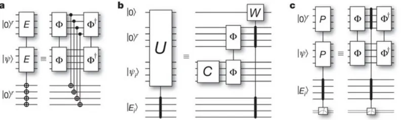
4.1 Circuits for Each Step of the Quantum Metropolis Algorithm. a, This subfigure depicts the initial application of the quantum phase estimation algorithm. The input is the initial guess for the ground state and two r-qubit registers. The quantum phase estimation circuit, represented by Φ in the diagram, acts on the state and the second register. The resulting energy is copied from the second register to the first register by a sequence of r CNOT gates. The inverse quantum phase estimation circuit, represented byΦ†, is then applied to the second register and the state. b, The quantum Metropolis circuit takes as its input the state, one r-qubit register initialized to |0ir, and a single qubit register initialized to |0i. The circuit can be separated into the local unitary operator C, which acts upon the state, and two quantum phase estimation gates, which act upon both the state and the r-qubit register. The quantum Metropolis gate acts upon the single-qubit register |0i. c, The operations required for returning to the original state if the update is rejected are shown in this subfigure. The quantum phase estimation gate is applied to both the state and the new r-qubit register; once the energy is compared to the original energyEi, the quantum phase estimation can be undone with inverse quantum phase estimation gates. Reprinted by permission from Macmillan Publishers Ltd: Nature471:87, copyright 2011. . . . 24 4.2 A single application of the quantum Metropolis map. The circuit

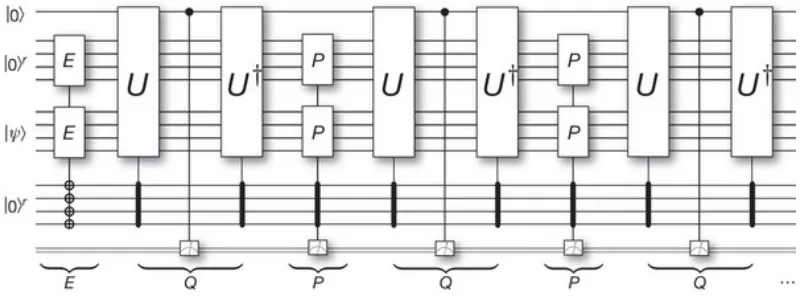
for a single application of the quantum Metropolis stochastic map is presented above. The two gates E act on the state |ψiand the r-qubit register prepare the eigenstate as the input of the algorithm. The first U gate proposes an update; the first Q measurement determines whether it is accepted or rejected. Should the update be rejected, then the P measurement will be performed. The alternating measurements of Q and P will continue until a positive measurement outcome of

(7)

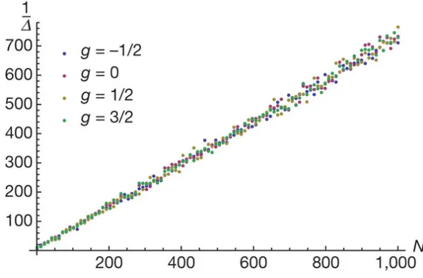
6.1 Inverse spectral gap of the quantum Ising model’s quantum Metropolis map. The inverse spectral gap of the quantum Ising model’s quantum Metropolis stochastic map, 1/∆, has been plotted as a function of N, the number of spins in the system. The quan-tum Ising model can be represented as the following Hamiltonian:

Í

k XkXk+1+YkYk+1+gZk. A single spin flip is used as the update rule. The linear relationship indicates that the quantum Metropolis algorithm mixes in polynomial time for the specific quantum Ising model used. Reprinted by permission from Macmillan Publishers Ltd: Nature471:87, copyright 2011. . . 36 6.2 The spectral gap behavior is modeled for varying system size from

three to ten qubits for a fixed row sparsity of s = 1. The values of the nonzero elements were generated from a uniform distribution U(0,1). The mean spectral gaps for the different system sizes are used as the data points. We use a constant fit of y(x)= aand obtain

a=0.0588073,σa= 0.00368339, and χ2/(n−1)= 0.0582212. . . . 43 6.3 The spectral gap behavior is modeled for varying system size from

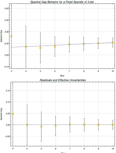
three to ten qubits for a fixed row sparsity of s = 3. The values of the nonzero elements were generated from a uniform distribution U(0,1). The mean spectral gaps for the different system sizes are used as the data points. We use a linear fit ofy(x)=a+bxand obtain

a=0.224419,σa =0.0620334,b=0.00286737,σb =0.00722124, and χ2/(n−2)= 0.0265796. . . 44 6.4 The spectral gap behavior is modeled for varying system size from

three to ten qubits for a fixed row sparsity ofs =3. The values of the nonzero elements were generated from a normal distributionN(0,1). The mean spectral gaps for the different system sizes are used as the data points. We use a linear fit of y(x) = a+ bx and obtain

(8)

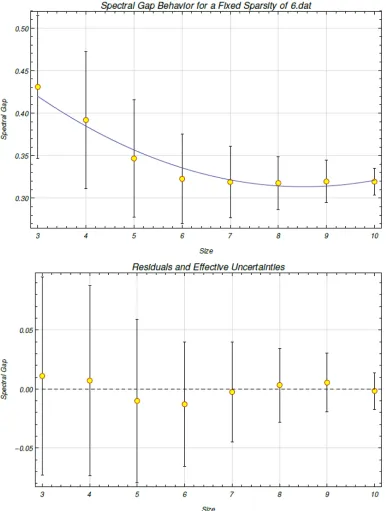
6.5 The spectral gap behavior is modeled for varying system size from three to ten qubits for a fixed row sparsity ofs =6. The values of the nonzero elements were generated from a uniform distributionU(0,1). The mean spectral gaps for the different system sizes are used as the data points. We use a quadratic fit of y(x)= a+bx+cx2and obtain

a = 0.566395, σa = 0.174746, b = −0.0593442, σb = 0.0485003,

c=0.00348011,σc= 0.00322192, and χ2/(n−3)= 0.0358664. . . 46 6.6 The spectral gap behavior is modeled for varying system size from

three to ten qubits for a fixed row sparsity ofs =6. The values of the nonzero elements were generated from a normal distributionN(0,1). The mean spectral gaps for the different system sizes are used as the data points. We use a quadratic fit of y(x)= a+bx+cx2and obtain

a = 0.560406, σa = 0.190018, b = −0.0624437, σb = 0.0533355,

c=0.00384023,σc= 0.00360865, and χ2/(n−3)= 0.0696112. . . 47 6.7 The spectral gap behavior is modeled for varying system size from

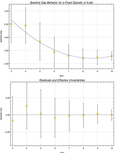
three to ten qubits for a fixed row sparsity ofs =8. The values of the nonzero elements were generated from a uniform distributionU(0,1). The mean spectral gaps for the different system sizes are used as the data points. We use a quadratic fit of y(x)= a+bx+cx2and obtain

a = 0.664627, σa = 0.159184, b = −0.0799266, σb = 0.0461287,

c=0.00463503,σc= 0.00314, and χ2/(n−3)=0.048682. . . 48 6.8 The spectral gap behavior is modeled for varying system size from

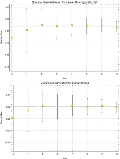
three to ten qubits for a linear row sparsity of s = n, wherenis the number of qubits. The values of the nonzero elements were generated from a uniform distribution U(0,1). The mean spectral gaps for the different system sizes are used as the data points. We use a constant fit of y(x) = a and obtain a = 0.320328, σa = 0.0133158, and

χ2_/(_n₋₁₎₌₀_._{027536. . . 50} 6.9 The spectral gap behavior is modeled for varying system size from

three to ten qubits for a linear row sparsity of s = n. The values of the nonzero elements were generated from a normal distribution N(0,1). The mean spectral gaps for the different system sizes are used as the data points. We use a constant fit of y(x)= aand obtain

(9)

6.10 The spectral gap behavior is modeled for varying system size from three to ten qubits for a quadratic row sparsity ofs= n2−4. The values of the nonzero elements were generated from a uniform distribution U(0,1). The mean spectral gaps for the different system sizes are used as the data points. We use a linear fit ofy(x)=a+bxand obtain

a=0.631437,σa=0.0467774,b= −0.0309497,σb =0.00580634, and χ2/(n−2)= 0.573525. . . 52 6.11 The spectral gap behavior is modeled for varying system size from

three to ten qubits for a quadratic row sparsity of s = n2 −n+ 1. The values of the nonzero elements were generated from a uniform distributionU(0,1). The mean spectral gaps for the different system sizes are used as the data points. We use a linear fit ofy(x)=a+bx

and obtain a = 0.626823, σa = 0.0421773, b = −0.0302081, σb = 0.0050857, and χ2/(n−2)= 0.480315. . . 53 6.12 The spectral gap behavior is modeled for varying system size from

three to ten qubits for a quadratic row sparsity of s = n2 −n+ 1. The values of the nonzero elements were generated from a normal distributionN(0,1). The mean spectral gaps for the different system sizes are used as the data points. We use a linear fit ofy(x)=a+bx

and obtain a = 0.648627, σa = 0.0538921, b = −0.0339071, σb = 0.00628929, and χ2/(n−2)= 0.409645. . . 54 6.13 The spectral gap behavior is modeled for varying system size from

three to ten qubits for a cubic row sparsity of s = b0.5n3− n2 −

n−2c . The values of the nonzero elements were generated from a uniform distributionU(0,1). The mean spectral gaps for the different system sizes are used as the data points. We use a quadratic fit of

y(x)= a+bx+cx2and obtaina = 0.274312, σa = 0.110236,b =

0.0844276, σb = 0.0317495, c = −0.00682071, σc = 0.00227522, and χ2/(n−3)= 1.41193. . . 55 6.14 The spectral gap behavior is modeled for varying row sparsity from

1 to 2n, wherenis the number of qubits, for a fixedn=6. We fit the model with the function y(x) = alog(bx)and obtaina = 0.105908,

σa= 0.00371134,b= 2.7578, andσb=0.368026. The p-values for

(10)

6.15 The spectral gap behavior is modeled for varying row sparsity from 1 to 2n, wherenis the number of qubits, for a fixedn=8. We fit the model with the functiony(x)= alog(bx)and obtaina =0.0637553,

σa= 0.00385493,b= 11.8402, andσb=4.61932. The p-values for

(11)

LIST OF TABLES

Number Page

C.1 Table of Spectral Gaps for a Constant Row Sparsity of 1. The spectral gaps of random Hamiltonians with varying system sizes and a constant row sparsity of one are recorded in this table. The Hamiltonians were generated using a uniform distribution, and the system sizes range from three to ten qubits. The spectral gaps for each size and row sparsity form a Gaussian distribution over the iterations; the values chosen to generate the plots are the means of the distribution. The standard deviations are recorded in this table for bookkeeping purposes. . . 71 C.2 Table of Spectral Gaps for a Constant Row Sparsity of 3

(Uni-form). The spectral gaps of random Hamiltonians with varying system sizes and a constant row sparsity of three are recorded in this table. The Hamiltonians were generated using a uniform distribution, and the system sizes range from three to ten qubits. The spectral gaps for each size and row sparsity form a Gaussian distribution over the iterations; the values chosen to generate the plots are the means of the distribution. The standard deviations are recorded in this table for bookkeeping purposes. . . 72 C.3 Table of Spectral Gaps for a Constant Row Sparsity of 3 (Normal).

(12)

C.4 Table of Spectral Gaps for a Constant Row Sparsity of 6 (Uni-form). The spectral gaps of random Hamiltonians with varying system sizes and a constant row sparsity of six are recorded in this table. The Hamiltonians were generated using a uniform distribution, and the system sizes range from three to ten qubits. The spectral gaps for each size and row sparsity form a Gaussian distribution over the iterations; the values chosen to generate the plots are the means of the distribution. The standard deviations are recorded in this table for bookkeeping purposes. . . 73 C.5 Table of Spectral Gaps for a Constant Row Sparsity of 6 (Normal).

The spectral gaps of random Hamiltonians with varying system sizes and a constant row sparsity of six are recorded in this table. The Hamiltonians were generated using a normal distribution, and the system sizes range from three to ten qubits. The spectral gaps for each size and row sparsity form a Gaussian distribution over the iterations; the values chosen to generate the plots are the means of the distribution. The standard deviations are recorded in this table for bookkeeping purposes. . . 73 C.6 Table of Spectral Gaps for a Constant Row Sparsity of 8. The

spectral gaps of random Hamiltonians with varying system sizes and a constant row sparsity of eight are recorded in this table. The Hamiltonians were generated using a uniform distribution, and the system sizes range from three to ten qubits. The spectral gaps for each size and row sparsity form a Gaussian distribution over the iterations; the values chosen to generate the plots are the means of the distribution. The standard deviations are recorded in this table for bookkeeping purposes. . . 74 D.1 Table of Spectral Gaps for a Linear Row Sparsity (Uniform). The

(13)

D.2 Table of Spectral Gaps for a Linear Row Sparsity (Normal). The spectral gaps of random Hamiltonians with varying system sizes and a linear row sparsity of s = n are recorded in this table. The Hamiltonians were generated using a normal distribution, and the system sizes range from three to ten qubits. The spectral gaps for each size and row sparsity form a Gaussian distribution over the iterations; the values chosen to generate the plots are the means of the distribution. The standard deviations are recorded in this table for bookkeeping purposes. . . 76 D.3 Table of Spectral Gaps for a Quadratic Row Sparsity with No

Lin-ear Term. The spectral gaps of random Hamiltonians with varying system sizes and a quadratic row sparsity ofs =n2−4 are recorded in this table. The Hamiltonians were generated using a normal distribu-tion, and the system sizes range from three to ten qubits. The spectral gaps for each size and row sparsity form a Gaussian distribution over the iterations; the values chosen to generate the plots are the means of the distribution. The standard deviations are recorded in this table for bookkeeping purposes. . . 76 D.4 Table of Spectral Gaps for a Quadratic Row Sparsity (Uniform).

The spectral gaps of random Hamiltonians with varying system sizes and a quadratic row sparsity of s = n2−n+1 are recorded in this table. The Hamiltonians were generated using a uniform distribution, and the system sizes range from three to ten qubits. The spectral gaps for each size and row sparsity form a Gaussian distribution over the iterations; the values chosen to generate the plots are the means of the distribution. The standard deviations are recorded in this table for bookkeeping purposes. . . 77 D.5 Table of Spectral Gaps for a Quadratic Row Sparsity (Normal).

(14)

D.6 Table of Spectral Gaps for a Cubic Row Sparsity. The spectral gaps of random Hamiltonians with varying system sizes and a cubic row sparsity of s = b0.5n3−n2−n−2c are recorded in this table. The Hamiltonians were generated using a uniform distribution, and the system sizes range from four to ten qubits. The spectral gaps for each size and row sparsity form a Gaussian distribution over the iterations; the values chosen to generate the plots are the means of the distribution. The standard deviations are recorded in this table for bookkeeping purposes. . . 78 E.1 Table of Spectral Gaps for Varying Sparsity at 6 Qubits. The

spectral gaps of random Hamiltonians with varying row sparsities for a fixed system size of six qubits are recorded in this table. The Hamiltonians were generated using a uniform distribution. The spec-tral gaps for each size and row sparsity form a Gaussian distribution over the iterations; the values chosen to generate the plots are the means of the distribution. The standard deviations are recorded in this table for bookkeeping purposes. . . 79 E.2 Table of Spectral Gaps for Varying Sparsity at 8 Qubits. The

(15)

NOMENCLATURE

Affine function. A function composed of a linear function followed by its transla-tion..

Completely positive map. A mapping describing quantum evolution by mapping from a set of density matrices onto itself..

Frustration free system. A system whose Hamiltonian can be written as the sum of terms whose ground states match that of the Hamiltonian..

Hilbert space. The configuration space of a quantum system..

Phase space. A multidimensional space that contains all of the particle’s possible states, which are characterized by position and momentum..

Positive semidefinite matrix. A Hermitian matrix with nonzero eigenvalues.. Slater’s condition. A sufficient condition that a primal problem must satisfy if

strong duality is to hold. The condition holds if the primal problem is strictly feasible; the weak form of the condition allows a relaxation of the strictly feasible rule if the function in question is affine..

Sparsity pattern. An explicitly defined pattern of nonzero elements in a matrix.. Spectral gap. The largest difference between the eigenvalues of the map..

Spectral norm. The square root of the maximum eigenvalue of a matrix.. Stochastic map. A completely positive map that also preserves the trace.. Strong duality. A condition under which the duality gap is zero..

(16)

C h a p t e r 1

INTRODUCTION

The concept of quantum computers was born in 1981, when Feynman presented the difficulties of simulating quantum systems with classical approximations. In his seminal lecture on simulating physics with computers, he posed a question to physi-cists: is it possible to build a computer in which the elements required to simulate a physical system is proportional to the space-time volume of the system? Such a computer wouldn’t be classical – quantum mechanics is inherently probabilistic, but simulating probabilities for large physical systems is an intractable problem for classical computers. If a classical computer is asked to calculate all of the pos-sible configurations of R particles for N points in space, then the computer must be able to hold NR configurations – something that cannot be done by a computer of order N. For realistic physical systems, the number of particles is on the same order of the number of points in space – in such cases, the computer must hold

NN elements. Feynman concluded that if a polynomial increase in the size of a physical system results in an exponential increase of required computing elements, then a classical computer can’t efficiently simulate quantum physics by computing the evolution of a wavefunction [1]. Could a classical computer imitate the be-havior of quantum mechanics by directly generating the probabilities encountered in nature? The probability of finding a classical particle at a certain point in the phase space is characterized by the phase-space probability distribution, which is non-negative and yields one when integrated over the phase space. The counterpart to the classical phase-space probability distribution in the quantum domain is the Wigner quasiprobability distribution. The Wigner function gives the probability of locating a particle atxwhen it is integrated over momentum, and it gives the momen-tum distribution when it is integrated over position [2]. However, the results of the Wigner quasiprobability distribution cannot be interpreted as probabilities, because the Wigner function admits negative values – how would negative probabilities be interpreted [3]?

(17)

(18)

1.1 Applications to Traditional Computing

Up until now, we have limited our discussion of the practical applications of quantum computers to simulating quantum physics. However, the influx of quantum algo-rithms – namely, algoalgo-rithms that run on quantum computers – has piqued interest in applying quantum computing techniques to problems in classical computer science. One class of algorithms of particular interest to our research is the quantum Gibbs sampler – a class of quantum Markov chain Monte Carlo algorithm that allows random samples to be generated from arbitrary distributions without calculating the probability density function [5]. Gibbs sampling is primarily used in physics to find a statistical ensemble’s Gibbs state, or the system’s equilibrium distribution that remains stationary under further evolution. Since it is a statistical technique, it can be utilized in any statistical context, and thus plays a role in solving convex optimization problems. Convex optimization is a category of problems that can be solved by minimizing a convex function over a convex set – practical applications of convex optimization range from operations research to communications to con-trol systems to finance. We limit ourselves to discussing the application of Gibbs sampling to semidefinite programming, a subfield of convex optimization that min-imizes a linear function over the cone defined by a linear combination of positive semidefinite matrices with coefficients that add up to one.

(19)

quantum computer [8]. The quantum Metropolis stochastic map can be simulated classically by performing a random walk on the Hamiltonian’s eigenstates, discard-ing rejections, and accountdiscard-ing for all possible consecutive moves. The spectral gap of the resulting map is shown to be inversely proportional to the running time of the quantum algorithm; in our case, the map is represented as 2Nx2N matrix, where N is the number of qubits in the system, and the spectral gap is the difference between the largest and the second largest eigenvalues. Thus, a program hoping to model the running time of the quantum Metropolis sampling algorithm as a function of system size or sparsity must compute the spectral gap for random Hamiltonians. While the quantum Metropolis algorithm has been shown to increase linearly in the system size, our study focuses on Hamiltonians generated randomly from normal distributions. While there is no guarantee that the algorithm will yield exponential speedups for arbitrary local Hamiltonians – indeed, the recent work of Brandão and Svore only demonstrate that a quadratic speedup can be achieved for quantum semidefinite programming with existing quantum Gibbs samplers [7] – the linear combinations of the constraint matrices used in semidefinite programming are best represented as randomly generated Hamiltonians.

The focus of this thesis is to observe and discuss the effects that preparing the Gibbs states on a quantum computer has on the performance of classical semidefinite programming with the matrix multiplicative weights update method. Since the update step is prepared by Gibbs sampling, the running time of the quantum Gibbs sampler dominates the quantum semidefinite programming algorithm’s running time, and thus an exponential speedup in the preparation of Gibbs states on a quantum computer will result in an exponential speedup in semidefinite programming. The numerical simulations of the running time of a quantum Gibbs sampler – in this case, the quantum Metropolis algorithm by Temmeet al. – for different system sizes and different sparsities will shed light on the question of whether there exists certain circumstances under which the Gibbs states of randomly generated Hamiltonians are prepared exponentially faster on a quantum computer.

References

1_{R. P. Feynman, “Simulating physics with computers”, International Journal of} Theoretical Physics21, 467–488 (1982).

(20)

3_{J. E. Moyal, “Quantum mechanics as a statistical theory”, Mathematical} Proceed-ings of the Cambridge Philosophical Society45, 99–124 (1949).

4_{S. Lloyd, “Universal quantum simulators”, Science}_{273, 1073–1078 (1996).} 5_{G. Casella and E. I. George, “Explaining the gibbs sampler”, The American}

Statistician46, 167–174 (1992).

6_{S. Arora and S. Kale, “A combinatorial, primal-dual approach to semidefinite} programs”, Journal of the ACM46, 12.1–12.35 (2016).

7_{F. Brandão and K. Svore, “Quantum speed-ups for semidefinite programming”,} (2016), arXiv:1609.05537 [quant-ph].

(21)

C h a p t e r 2

CLASSICAL SEMIDEFINITE PROGRAMMING

Before the quantization of the semidefinite programming algorithm can be discussed, we must clarify what Arora’s and Kale’s combinatorial, primal-dual semidefinite programming entails. We use Arora’s and Kale’s definition of a primal-dual algo-rithm – that is, an algoalgo-rithm that gives both primal and dual solutions, and bounds the duality gap, or the difference between the two solutions, with weak duality. Weak duality states that the duality gap is always greater than or equal to zero, which indicates that the primal solution is always greater than or equal to the dual solution [1]. For a general semidefinite program withn2variables andmconstraints, the primal problem is generally formulated as the following [2].

max tr(CX)

∀j ∈ [m]: tr(AjX) ≤bj

X 0

The corresponding dual problem is as follows [2].

min by

m Õ

j=1

Ajyj C

y≥ 0

We can convert a semidefinite program given in the primal form to the dual form and vice versa. We observe that the n2 variables are presented as a nxn positive semidefinite matrixX. Because there aremconstraints, there arem nxnHermitian matricesAj for j ∈ [m]. The matrixCis a nxnpositive-semidefinite matrix. For

the dual program, the dual variables are held in the vectory=< y1,y2, ...,ym >and

(22)

2.1 Arora-Kale Algorithm for Semidefinite Programming

The Arora-Kale algorithm for semidefinite programming seeks a primal feasible solution to a primal-dual semidefinite program; simultaneously, it attempts to in-crementally build a dual solution with the help of an auxiliary function called the ORACLE. It takes as its initial inputs the following parameters: α, which serves as a guess for the optimum value of the solution; an error parameter represented by an arbitrarily small constant >0; a width parameter ρ ≥ 0 for theORACLE; and a scaling constraint R [2]. By taking A1 = I and b1 = R, Arora and Kale guarantee that tr(X) ≤ R, which gives a constraint that bounds the feasible region of the semidefinite program [2]. Furthermore, settingA1 = Iallows us to find values

y1,y2, ...ym > 0 that satisfyAjyj C. The weak form of Slater’s condition then

holds, ensuring that strong duality holds in our semidefinite program. Thus the duality gap is zero, and the primal problem and the dual problem share the same optimum solution [3]. Nevertheless, in order to account for error, we introduce as the gap between the primal feasible solution and the dual feasible solution. The algorithm is searching for a positive semidefinite matrix as a primal feasible solution that is≥ α– ifORACLEnever fails, then the algorithm successfully yields a dual feasible solution that is≤ α+ [2].

The parameterαbounds the range thatORACLEsearches – it appears as a constraint on the vector y outputted by the ORACLE. The width parameter ρ is defined as the smallest nonnegative value that bounds the ORACLE’s output y such that ||Ajyj − C|| ≤ ρ. The significance of the width parameter is twofold: ρ serves

as both a measure of progress and a scaling factor for the loss matrices M that guarantee the spectral norm ofM is bound by one. A large width would indicate that the ORACLEhas not been effective in helping the algorithm make progress. The loss matrixMis required to perform the matrix multiplicative weights update step, as are the other parameters and R. The last two parameters are gathered withρandαinto a new parameter, which plays a role in the matrix multiplicative weights algorithm.

The ORACLE

(23)

ORACLE based on whether the problem is a maximization semidefinite program or a minimization semidefinite program. We reproduce their definitions here: Definition 2.1(ORACLEfor Maximization Semidefinite Programs) For maximiza-tion semidefinite programs, the auxiliary algorithmORACLEmust be constructed so that it takes as its input a positive semidefinite matrix X 0, or the candidate primal solution, and tries to output a vectorythat meets the following constraints:

b·y≤ α

m Õ

j=1

tr(AjX)yj ≥ tr(CX)

y≥ 0

If no such vectory exists, then theORACLEoutputsFAIL and returnsX. Arora and Kale prove that if theORACLEfails, then an appropriately scaledXis a primal feasible solution≥ α. But if ayis found, then the current candidate primal solution X fails as the primal feasible solution, and the algorithm must proceed with its iterations. If the ORACLE never fails for T iterations, where T is determined by the matrix size and the four parameters defined earlier, then the algorithm outputs a dual feasible solution.

The definition of theORACLEfor minimization semidefinite programs is similarly constructed and reproduced below:

Definition 2.2(ORACLEfor Minimization Semidefinite Programs) For maximiza-tion semidefinite programs, the auxiliary algorithmORACLEmust be constructed so that it takes as its input a positive semidefinite matrix X 0, or the candidate primal solution, and tries to output a vectorythat meets the following constraints:

b·y≥ α

m Õ

j=1

tr(AjX)yj ≤ tr(CX)

y≥ 0

(24)

than reproduce the proof of the algorithm and the required lemmas below, we will point interested readers in the direction of the original paper [2]. But we will delve into a discussion of the mechanisms used in their paper, especially the mechanisms that are crucial to developing the quantum version of this algorithm.

Matrix Multiplicative Weights Algorithm

The backbone of the Arora-Kale primal-dual algorithm for solving semidefinite programs is the matrix multiplicative weights algorithm, which takes as its input the number of iterations T and a parameter , and uses the density matrix P(t) created from the previous weight matrixW(t), along with a loss matrix generated by an external sourceM(t), to output a new weight matrixW(t+1). This final matrix is responsible for updating the algorithm. The superscript (t) denotes the current iteration. The algorithm in its entirety is reproduced below from [2]:

Algorithm 1 (Matrix Multiplicative Weights Algorithm)

Letη ≤ 1. LetT be the number of iterations. Fort =1, ...,T:

1. Find the density matrixP(t) = W(t) tr(W(t)).

2. Find the loss matrix M(t)from the external source.

3. Compute the weight matrix for the next iteration:

W(t+1) =exp

−η(Ít_τ−₌₁1M(τ)).

(25)

Theorem 2.1: For any collection of loss matrices {M(1),M(2), ...M(T)}, the ma-trix multiplicative weights algorithm generates a collection of density matrices {P(1),P(2), ...P(T)}that satisfies the following inequality:

tr

T Õ

t=1

M(t)P(t)

!

≤ λn(

T Õ

t=1

M(t))+η

T Õ

t=1 tr

(M(t))2P(t)

+ log_ηn (2.1)

Corollary 2.2: For any collection of loss matrices {M(1),M(2), ...M(T)}, the ma-trix multiplicative weights algorithm generates a collection of density matrices {P(1),P(2), ...P(T)}that satisfies the following inequality:

tr

T Õ

t=1

M(t)P(t)

!

≤ λn(

T Õ

t=1

M(t))+ηT+ logn

η (2.2)

We will not reproduce the proofs, but we will discuss the significance of the derived conclusions to the final algorithm. In the Arora-Kale primal-dual algorithm for solving semidefinite programs, we have η = ₂_ρR and T = d4ρ2R2₂log(n)e. The main algorithm uses the slack matrix M(t) = Ím_j₌₁Ajyj − C as the loss matrix

during the matrix multiplicative weights update step. The slack matrix does not represent loss; mathematically speaking, it encodes the structure of the polytope D_α = y:y ≥ 0,b·y ≤ α for maximization problems, and of the polytope D_α = y:y≥ 0,b·y≥ α [5]. The slack matrix can also be intuitively interpreted as a matrix that represents the dual constraints [2]. The goal of the main algorithm is to produce such a dual feasible solutionythat the slack matrix is positive semidefinite – this is a costly task, so rather than pursue this goal directly, the algorithm uses the ORACLEto seek a slack matrix that has a nonnegative matrix inner product with X(t) = RP(t), the candidate primal solution that is updated iteratively along with the density matrices. This reduces the semidefinite dual problem to a linear program with two nontrivial constraints, which is an easier problem to solve [2].

(26)

The Primal-Dual Solver

We have discussed the matrix multiplicative weights update method and theORACLE in depth. These two auxiliary algorithms are the key mechanisms of the main al-gorithm: the matrix multiplicative weights update method urges the slack matrix in the positive semidefinite direction, which speeds up the search for a dual feasible solution, and the ORACLE checks iteratively which solution – primal or dual – is close to feasibility. TheORACLE may not necessarily output the dual feasible solution even when such a solution exists – in cases when the candidate primal solution has become almost primal feasible, but the dual feasible solution has not been reached yet, theORACLE may choose to fail and simply output the primal feasible solution [2].

(27)

Algorithm 2 (Arora-Kale Semidefinite Programming Algorithm (2016))

Set X(1) = R_nI. Let T be the number of iterations. We have η = ₂_ρR and T =

d4ρ2R2₂log(n)e. Fort =1, ...,T:

1. Run the matrix multiplicative weights algorithm and find the density matrix

P(t).

2. SetX(t) = RP(t).

3. InputX(t) intoORACLEand run the auxiliary algorithm.

4. IfORACLE fails, then abort and return X(t). Otherwise, store the results

obtained as vectory(t).

5. Compute the loss matrix M(t) = Ím_j₌₁Ajyj−C and feed it into the matrix

multiplicative weights algorithm for the next iteration.

6. IfORACLEdoesn’t fail for T iterations, then output the dual feasible solution ¯

y= _T1ÍT_t₌₁y(t)+ _Re1, wheree1=< 1,0, ...0 >T∈ Rm.

Brandãoet al. uses the 2007 version of the Arora-Kale algorithm for their quantum semidefinite programming algorithm, where the parameters are defined in a slightly different way. The error parameter is defined asδ, such that the dual feasible solution is at most (1+ δ)α, and what is defined asη in the 2016 publication is separated into two parameters and0in the 2007 proceedings paper. We reproduce the 2007 version of the matrix multiplication weights algorithm from [6]:

Algorithm 3 (Matrix Multiplicative Weights Algorithm)

Let < 1

2 and let

0 ₌ ₋

log(1− ). Let T be the number of iterations. For t =1, ...,T:

1. Compute the weight matrix: W(t) =exp−0(Ít_τ−₌1₁M(τ)). 2. Find the density matrixP(t) = W(t)

tr(W(t)).

(28)

The main algorithm witnesses one more change in its transformation from the 2007 version to the 2016 version: in its previous incarnation, the loss matrix was defined asM(t) =

Ím

j=1Ajyj−C+ ρI

/2ρ. The full algorithm is reproduced below from [6]:

Algorithm 4 (Arora-Kale Semidefinite Programming Algorithm (2007))

Set X(1) = R_nI. Let T be the number of iterations. We have = ₂δα_ρR and 0 =

−log(1−). In addition, we letT = ρ2R_δ22log_α2(n). Fort = 1, ...,T:

1. InputX(t) intoORACLEand run the auxiliary algorithm.

2. IfORACLE fails, then abort and return X(t). Otherwise, store the results

obtained as vectory(t).

3. Compute the loss matrix M(t) = Ím_j₌₁Ajyj−C and feed it into the matrix

multiplicative weights algorithm for the next iteration.

4. Run the matrix multiplicative weights algorithm and find the density matrix

P(t).

5. SetX(t) = RP(t).

6. IfORACLEdoesn’t fail for T iterations, then output the dual feasible solution ¯

y= _T1ÍT_t₌₁y(t)+ δα_Re1, wheree1=< 1,0, ...0 >T∈ Rm.

The worst case running time for the algorithm above is ˜Oρ2R_δ2₂mns, wheremis the number of input matricesAj,nis the dimension of the input matrices, andsis the

(29)

a quantum computer to prepare the Gibbs states of the Hamiltonians constructed by the linear combinations of the program’s input matrices [7]. Thus the numerical results of our runtime simulations for the quantum Metropolis algorithm will have implications for classical semidefinite programming algorithms that are not neces-sarily primal-dual but use the matrix multiplicative weight algorithm, such as the ones outlined by Penget al. [8]and Allen-Zhuet al. [9].

References

1_{E. de Klerk,}_{Aspects of semidefinite programming: interior point algorithms and} selected applications(Kluwer Academic Publishers, Dordrecht, The Netherlands, 2002).

3_{S. Boyd and L. Vandenberghe,}_{Convex optimization}_{(Cambridge University Press,} Cambridge, UK, 2004).

4_{S. Arora, E. Hazan, and S. Kale, “The multiplicative weights update method: a} meta-algorithm and applications”, Theory of Computing8, 121–164 (2012). 5_{R. Z. Robinson, “The positive semidefinite rank of matrices and polytopes”, PhD}

thesis (University of Washington, 2014).

6_{S. Arora and S. Kale, “A combinatorial, primal-dual approach to semidefinite} programs”, Proceedings of the 39th ACM Symposium on Theory of Computing (STOC’07), 227–236 (2007).

8_{R. Peng, K. Tangwongsan, and P. Zhang, “Faster and simpler width-independent} parallel algorithms for positive semidefinite programming”, (2016), arXiv:1201. 5135 [cs.DS].

(30)

C h a p t e r 3

QUANTUM SEMIDEFINITE PROGRAMMING

As in the classical version of the algorithm, the quantum semidefinite programming algorithm proposed by Brandãoet al. takes inm+1n×nconstraint matrices, finds the optimal values of primal and dual problems presented in the previous chapter, and outputs the primal feasible solution and/or the dual feasible solution. However, while the classical algorithm takes in the input matrices through the loss matrix

M(t), the quantum algorithm uses a different method to access the input matrices. In [1], there are two methods of accessing the input matrices. The first method is to define an oracle that takes as its input the index j denoting the constraint matrix

Aj, the index k ∈ [n]denoting the row of Aj, andl ∈ [s]denoting the number of nonzero elements in row k, wherel ≤ s, and outputs a bit string representation of the l −t h non-zero element in the k − t hrow in the j −t h constraint matrix Aj, which would yield the following map:

|j,k,l,zi → |j,k,l,z⊕ (Aj)_{k f}_jk(l)i, (3.1)

where fj k(l)is a function that outputs the column index corresponding to the position of thel−t hnonzero element in thek−t hrow ofAj.

The second method is more complicated and rests on the spectral decomposition of

Ai. We define two sets of oracles: the first set takes in the input matricesAi, prepares their eigenstates, and uses oracles to access their eigenvalues and the numbers bi. The decomposition of the input matrixAiis: Ai =Íri

l=1κ

i l|η

i li hη

i

l|. The valueriwill

be defined shortly. The second set of oracles only contains one oracle, which takes as its input(i,l), where i takes on the role of row index, and ri := λtr(Aiρ)+ µbi for real numbersλandµ, and quantum state ρ; the oracle outputs an approximation of Aj’s eigenstate |ηi

li and the corresponding eigenvalue κ i

l up to an error ν. The

valueri is defined such that it is the i-th eigenvalue of the Hamiltonian defined as

H(ρ, λ, µ):= Ím_i₌₁ri|ii hi|[1].

(31)

result in the interest of efficiency – it yields an estimated optimal value, an estimated ||y||₁and/ortr(X), and samples from y/||y||₁and/or from ρ:= X/tr(X).

The essence of the algorithm is that the time-consuming linear programs and matrix exponentials in the classical algorithm [2, 3] are replaced with Gibbs states prepared on a quantum computer, a replacement that offers a quantum speedup. The Gibbs samplers used to prepare the Gibbs states may range from [4–8], although Brandão et al. express hope that the quantum Metropolis sampling algorithm by Temme et al. [7] may work best heuristically. Brandão et al. noted that the density matrix generated with the matrix exponential of the loss matrix using the matrix multiplicative weights method from [3] can be replaced with a Gibbs state of a Hamiltonian composed from a linear combination of the input matrices [1]. They also demonstrate how the output of the classical oracle in [2, 3] can be approximated with a Gibbs state using a modified version of Jayne’s principle of maximum entropy [9, 10], which we reproduce from [10] with modifications from [1]:

Lemma 3.1(Lemma 4.6 from [10]) LetM(_Cn₎_{be the set of Hermitian matrices over} Cn, and D(Cn) be the set of density matrices over Cn. We define T ⊆ M(Cn)as

compact set of matrices and define∆T := sup_A∈T||A||. Defineπ ∈ D(Cn). Finally,

define γ = d_κ8₂log(m)∆(T)2e. We define one more input parameter κ. Then for everyκ > 0, there exists a set of matrices X1, ...,Xγ ∈ T such that:

˜

π :=

exp− κ 4∆(T)2

Íγ i=1Xi

tr exp − κ 4∆(T)2

Íγ i=1Xi

(3.2)

is bounded by [π −π˜]T ≤ κ. It should be obvious by now that κ is related to the

error parameterν in our case.

Brandãoet al. then adapt this lemma so that the output of theORACLE(ρ)becomes:

qρ,λ,ν(i):= exp(λtr(Aiρ)+ µ

Í ibi) Í

iexp(λtr(Aiρ)+ µÍibi)

. (3.3)

The constantsλ andν are reparameterized into k so that for an integer k we have [1]:

λ=− κ

(32)

ν =− κ

4R2(γ−k), (3.5)

and

γ = d 8

κ2log(m)R 2_e_.

(3.6) As in the classical algorithm,Ris the upper bound on the trace of the primal optimal solution [1]. We can now write qρ,λ,ν as qρ,k. We then give the definition that Brandãoet al. use for a Gibbs sampler.

Definition 3.2(Gibbs Sampler) A quantum circuit that takes as its inputν, a Hamil-tonian H, and an oracle to access the entries of H [11], and outputs a state ρthat obeys the constraint||ρ−eH/tr(eH)||₁ ≤ ν.

We see then that the output of the ORACLE used in [2, 3] can be approximated with Gibbs sampling. We won’t reproduce the algorithm in [1] for instantiation of ORACLE(ρ) through sampling, but it should be noted that the algorithm samples from distributions ¯qρ,k that are close in variational distance toqρ,k rather than from

qρ,k itself.

(33)

Algorithm 5 (Brandão-Svore Quantum SDP Algorithm (2016))

Oracles for accessing{A1, ...Am,C}where||C||,||Ai|| ≤ 1. Oracles for accessing

{b1, ...,bm} where bi ≥ 1. Parameter R where R is the upper bound on the

trace of the primal optimal solution. Parameterα, which a guess for the optimal solution, and the error δ > 0 such that that dual feasible solution is at most

α(1+δ). A free parameter Ξthat features in the lower bound on the probability of success: 1− O(exp(−logΞ(nm))). Set ρ(1) = _nI, = δ

28R2,

0₌ ₋_ln₍

1−), M =

80 log1+Ξ(8R2nm/)/2, L = 80 log1+Ξ(nm)/2, and Q = (10R)6ln2+Ξ(nm)/4. Setγ = d8₂ log(m)R2e. DefineGH(ρ) as the maximum number of calls made by the Gibbs sampler to the oracle that accesses the entries of H(ρ,k) for k ∈ [γ]. LetT be the number of iterations. SetT = 500R_δ32ln(n). Fort =1, ...,T:

1. Sety(t) =(0, ...0).

2. For k = 1, ..., γ and N = 1, ...,dαe, use the Gibbs sampler on H(ρ,k) to create M copies of q with up to an error of /4. Obtain M

inde-pendent samples {i1, ...iM} from q. Using (M + 1)L samples from ρ(t),

approximate {tr(Ai₁ρ(t)), ...,tr(Ai_Mρ(t)),tr(Cρ(t))} up to accuracy /2 and store the results as {ei₁, ...,ei_M},f. If 1/MÍM_j₌₁eij ≥ f/(N) − and 1/MÍM

j=1bij ≤ α/(N) + R, then set kt = k, Nt = N, q(t) = q, and

y(t) = Nq(t).

3. Abort and indicate failure if y(t) =(0, ...,0).

4. Use the Gibbs sampler onH(ρ(t),kt)to createQ+1copies ofq(t)with up to

an error of/4.

5. ObtainQindependent samples{i1, ...iQ} fromq(t). 6. ComputeM(t) = NtQ

−1ÍQ

j=1Ai j−C+2αI

4α .

7. DefineCt := 10 log2(m) γα

M+Q

GH(ρ(t)₎₊ 2γα

M Land the Gibbs sampler

on−0Ít_τ₌₁M(τ)

with an error up to/4to makeCt copies ofρ(t+1).

If the algorithm runs without failing, then it will output ||y¯||₁ and a sample from ¯

y/||y¯||₁ for ¯y = ₂δα_Re1+ _T1ÍTt=1y

(t)_{, where}

(34)

quantum speedups that have been rigorously verified in Brandãoet al. The quantum semidefinite programming algorithm by Brandão et al. has a worst case runtime ofn12m

1

2spoly(log(n),log(m),R,1/δ), where we once again emphasize thatnis the

dimension of the input matrices and thus the Hilbert space dimension and s is the row sparsity of the input matrices. The quantum algorithm offers a square root speedup in n and m over classical methods; Brandão et al. demonstrate that this is the best possible runtime in terms of n and m and give a lower bound for the complexity of the algorithm: Ω(n12 +m12) for a given (s, δ,R). However, there is

one case in which the algorithm can witness exponential speedups inn– when the quantum Gibbs states used in the algorithm can be efficiently prepared on a quantum computer [1].

While there is no way to rigorously prove that using the quantum Metropolis sam-pling scheme [7] to prepare the required Gibbs states will exponentially speed up the quantum semidefinite programming algorithm by Brandão et al. for arbitrary row-sparse Hamiltonians, we seek to demonstrate numerically that for three to ten qubits, the quantum semidefinite programming algorithm experiences an exponen-tial speedup in n when the quantum Metropolis algorithm is the chosen Gibbs sampler.

References

3_{S. Arora and S. Kale, “A combinatorial, primal-dual approach to semidefinite} programs”, Proceedings of the 39th ACM Symposium on Theory of Computing (STOC’07), 227–236 (2007).

4_{A. N. Chowdhury and R. D. Somma, “Quantum algorithms for gibbs sampling} and hitting-time estimation”, (2016), arXiv:1603.02940 [quant-ph].

5_{M. J. Kastoryano and F. G. S. L. Brandão, “Quantum gibbs samplers: the} com-muting case”, Communications in Mathematical Physics344, 915–957 (2016). 6_{D. Poulin and P. Wocjan, “Sampling from the thermal quantum gibbs state and}

evaluating partition functions with a quantum computer”, Physical Review Letters 103, 220502 (2009).

(35)

8_{M. Yung and A. Aspuru-Guzik, “A quantum–quantum metropolis algorithm”,} Proceedings of the National Academy of Sciences, 754–759 (2012).

9_{E. T. Jaynes, “Information theory and statistical mechanics ii”, Physical Review} 108, 171–190 (1957).

10_{J. R. Lee, P. Raghavendra, and D. Steurer, “Lower bounds on the size of} semidefi-nite programming relaxations”, Proceedings of the 47th Annual ACM Symposium on Theory of Computing (STOC ’15), 567–576 (2015).

(36)

C h a p t e r 4

QUANTUM METROPOLIS SAMPLING

Metropoliset al. devised the Metropolis algorithm in 1953 to calculate the prop-erties of classical many-body systems with the Markov chain Monte Carlo method [1]; while ground-breaking for classical simulations, it was not until recently that attempts to generalize the algorithm to quantum systems have succeeded. Pre-vious quantum Monte Carlo methods failed after encountering fermionic systems and the related sign problem, a catchall phrase describing the complications and difficulty surrounding the evaluation of a highly oscillatory integral [2]. Long af-ter the publication of Lloyd’s paper on the viability of quantum computing, there was still a dearth of quantum algorithms that allowed the efficient preparation of a Hamiltonian’s thermal or ground state.

The quantum algorithms that did prepare ground states efficiently only worked for frustration free systems, which limited research to a subset of physical systems [3]. In 2000, Terhal and Divincenzo discussed sampling from a physical system’s thermal state using methods reminiscent of the classical Metropolis algorithm; however, they neglected to provide a way to circumvent the no-cloning problem, which posed an obstacle to the crucial rejection step in the Metropolis algorithm. Furthermore, computing the eigenvalues of the Hamiltonian with the Fourier transform, a step that makes up half of the algorithm, may require a runtime exponential in system size [4]. In 2005, Aspuru-Guzik et al. expanded the phase estimation algorithm developed by Abramset al. [5] into a quantum algorithm that prepares ground states of more general Hamiltonians; the stringent requirement that the variational state overlap greatly with the ground state nevertheless limits the algorithm’s range of applicability [6].

(37)

Hamil-tonian’s eigenstates, it dispenses with the sign problem, offering an exponential speedup to quantum algorithms still plagued with the task of dealing with negative statistical weights. Furthermore, Temme et al. gives a method of circumventing the no-cloning problem and resolving the issue of the rejection step; the analysis of the algorithm’s total runtime includes the runtime of the rejection procedure. The running time is bounded by a function of the quantum Metropolis stochastic map’s spectral gap; since the relationship between the spectral gap and the system size is unknown for random Hamiltonians, the quantum Metropolis algorithm does not have a running time that is explicitly defined in system size [7]. Thus the quantum Metropolis algorithm in theory may offer an exponentially faster method of preparing a quantum computer in the ground or thermal state of the physical system at hand.

4.1 The Algorithm

Before the quantum version of the classical Metropolis algorithm is presented, we must introduce the classical Metropolis sampling method. We use the simplest example presented in the original 1953 paper: a lattice of N points where the distances between all of the points are known, so that the potential energy of the systemEis easily calculated. Configurations with a probability of exp(−E/kT)are chosen beforehand and equally weighed. The particles are then moved randomly; after a move, the change of energy∆E is calculated. If∆E < 0, then the move has caused the system to shift to a state of lower energy – such a move is permitted and thus retained. But if∆E > 0, then the probability of such a move is exp(−E/kT) – an implementation of a probabilistic move can be done by randomly selecting a number from[0,1]and retaining the move if the number< exp(−E/kT)[1]. Temmeet al. have devised a quantum algorithm that performs the same procedure on a given Hamiltonian’s eigenstates. Instead of moving a particle to a new location, a random local unitary operator is selected to act upon the qubits; the acceptance and rejection terms remain the same as in the classical case. But in the quantum case, the difficulties are threefold: the algorithm has to account for computing the Hamiltonian’s eigenstates and their corresponding energies, undoing quantum transformations if the move is rejected, and proving that the desired Gibbs state is the stationary state of the Markov chain [7].

(38)

finding the phase of a unitary operator is equivalent to calculating the operator’s energy eigenvalue, the quantum phase estimation algorithm can be used to prepare a random eigenstate |ψii as the initial guess for the Hamiltonian’s ground state and calculate its energy, which is stored in an empty register, yielding |ψii |Eii. An implementation of the phase estimation algorithm can be found in [8]. A random local unitary operationCis then applied to the eigenstate, yieldingC|ψii =

Í

k xi_k|ψki. The quantum phase estimation algorithm is performed again to calculate

the energy of the new configuration, which is stored in the second register, yielding

Í

k xi_k|ψki |Eii |Eki.

If there were no rejection procedure, then we could proceed to measure the second register to find the energy and collapse the wavefunction. If this were a classi-cal algorithm, then we could store a copy of the original wavefunction so that we could simply return to it should the update be rejected; however, the no-cloning theorem rules out this possibility for quantum algorithms. Thus the quantum Metropolis circuit must include another gate – a gate that doesn’t perform a full energy measurement, but rather only slightly disturbs the state. The only infor-mation that is yielded by such a measurement is whether to accept or reject the update. A final register is introduced in this step, as the gate transforms the state into

Í k xi_k

q

f_ki|ψki |Eii |Eki |1i+Í k xi_k

q

1− f_ki|ψki |Eii |Eki |0i, where the amplitudes

x_ki q

f_ki are the quantum analog of the classical Metropolis transition probabilities. The function f_kiis f_ki = min(1,exp(−β(Ek −Ei))).

The quantum Metropolis circuit up to the rejection procedure can be summed up as [7]:

|ψii |Eii |0i |0i →C|ψii |Eii |0i |0i → Õ

k

xi_k|ψki |Eii |0i |0i

→ Õ

k

xi_k|ψki |Eii |Eki |0i

→ Õ

k xi_k

q

f_ki|ψki |Eii |Eki |1i+Õ

k xi_k

q

1− f_ki|ψki |Eii |Eki |0i

(39)

will then be fed into the algorithm again at the start of a new iteration. This measurement is denoted as Q. But if the outcome is |1i, then the move has been rejected and the algorithm must return to the original state [7]. In the case that the update is rejected, the algorithm can return to the original state using a procedure similar to the witness-preserving amplification scheme for QMA described in [9]. The circuits used to implement the quantum Metropolis algorithm are described in detail below in Fig. (4.1), which is reproduced from [7]:

Figure 4.1: Circuits for Each Step of the Quantum Metropolis Algorithm. a, This subfigure depicts the initial application of the quantum phase estimation algorithm. The input is the initial guess for the ground state and two r-qubit registers. The quantum phase estimation circuit, represented byΦin the diagram, acts on the state and the second register. The resulting energy is copied from the second register to the first register by a sequence of r CNOT gates. The inverse quantum phase estimation circuit, represented byΦ†, is then applied to the second register and the state. b, The quantum Metropolis circuit takes as its input the state, one r-qubit register initialized to |0ir, and a single qubit register initialized to |0i. The circuit can be separated into the local unitary operatorC, which acts upon the state, and two quantum phase estimation gates, which act upon both the state and the r-qubit register. The quantum Metropolis gate acts upon the single-qubit register|0i. c, The operations required for returning to the original state if the update is rejected are shown in this subfigure. The quantum phase estimation gate is applied to both the state and the new r-qubit register; once the energy is compared to the original energyEi, the quantum phase estimation can be undone with inverse quantum phase estimation gates. Reprinted by permission from Macmillan Publishers Ltd: Nature 471:87, copyright 2011.

(40)

two negatives is constant, so repeated applications of this sequence gives a success probability that exponentially approaches one [7]. The circuit for the rejection procedure can be found below in Fig. (4.2), which is reproduced from [7]:

Figure 4.2: A single application of the quantum Metropolis map. The circuit for a single application of the quantum Metropolis stochastic map is presented above. The two gates E act on the state |ψi and the r-qubit register prepare the eigenstate as the input of the algorithm. The first U gate proposes an update; the first Q measurement determines whether it is accepted or rejected. Should the update be rejected, then the P measurement will be performed. The alternating measurements of Q and P will continue until a positive measurement outcome ofP1is obtained. Reprinted by permission from Macmillan Publishers Ltd: Nature471:87, copyright 2011.

The possible results of the measurement, represented as the Hermitian projectors

Q0,Q1, P0, andP1are defined as below:

Q0=U†(I⊗I⊗I⊗ |0i h0|)U Q1=U†(I⊗I⊗I⊗ |1i h1|)U

P0=

Õ

i Õ

Eα,Ei

|ψαi hψα| ⊗ |Eii hEi| ⊗_I⊗_I

P1=

Õ

i Õ

Eα=Ei

|ψ_αi hψ_α| ⊗ |Eii hEi| ⊗_I⊗_I

It is obvious from the definition ofP1that ifP1is obtained, then the measurement P, as positioned in part c of Fig. (4.1), has compared the energy of the state to its original energy and found them to be the same.

(41)

came up with the concept of quantum detailed balance, which holds that if{ψi} is a set of complete basis states on a physical Hilbert space and{pi}is its probability distribution, then if a completely positive map E satisfies the following condition,

σ =Í

ipi|ψii hψi|is the map’s fixed point. The condition is as follows [7]:

√

pnpmhψi| E(|ψni hψm|) |ψji =√pipjhψm| E(|ψji hψi|) |ψni (4.1) This condition only guarantees that the Gibbs state is a possible fixed point of E – the uniqueness of the fixed point and the rate of convergence are dependent on the choice of updates{C} [7]. It is known from [10] that if the set of possible updates is chosen to be the universal gate set, then the completely positive mapEis ergodic, and the fixed point is unique. In our implementation, we choose the set of Pauli operators{I,X,Y,Z} as our set of possible updates{C}.

The runtime of the algorithm is given by the mixing time, or the number of times that the completely positive mapEmust be applied to reach the Gibbs state. Before we reproduce the mixing timemmi x, we first discuss the mixing error mi x used to bound the mixing time [7]:

||Emmix_[ρ

0] −σ∗||1 ≤ mi x (4.2)

In other words, the mixing error is defined as the upper bound of the trace norm distance of the completely positive map E. In the equation above, ρ0 is the initial state and σ∗ is the steady state. Since the trace norm distance is also bounded by the following equation [11]:

||Em[ρ] −σ∗||₁ ≤Cex p(1−∆)m, (4.3)

whereCex p is a constant that scales exponentially with the system size and∆is the spectral gap, or the difference between the largest and the second largest eigenvalues ofE, it is obvious that the mixing time is bounded as below [7]:

mmi x ≥ O

ln(1/mi x) ∆

(4.4)

(42)

explicitly defined. Thus there is no way to observe how the mixing time behaves as the system size increases. However, it is known that the classical Metropolis algorithm converges quickly if the physical system thermalizes – in fact, it may converge even more quickly, because the Metropolis algorithm is allowed to perform unphysical updates in its simulation of thermalization [7]. The resemblance between the classical and the quantum versions of the algorithm gives hope that the quantum Metropolis algorithm will behave similarly.

We now reproduce the entire algorithm from [7], assuming that no errors occur during quantum phase estimation:

Algorithm 6 (Quantum Metropolis Algorithm by Temmeet al.)

1. Initialize four quantum registers. The first will hold the quantum states. The second and third registers need to hold r-qubits and will respectively encode the energy of the original state and be used during quantum phase estimation. The last register only needs to hold a single qubit and is used to accept or reject the Metropolis update.

2. Reinitialize the last three ancillas and implement the circuit shown in part a of Fig. (4.1).

3. Define {C} such that the probability of randomly selectingC is the same

as selectingC†. Implement the circuit shown in part b of Fig. (4.1). For

energiesEiandEk, the unitaryW(Ei,Ek)is defined as:

W(Ei,Ek)=©

« q

1− f_ki q

f_ki q

f_ki −

q

1− f_ki ª ®

¬

(4.5)

4. Measure the last ancilla qubit. If the result is |1i orQ1, then the update is

accepted with probability∝ |xi_k q

f_ki|2, and the second ancilla qubit should be measured to obtain the energy required for a new iteration of the quantum Metropolis algorithm. If the result is |0i or Q0, then the update has been

rejected. ApplyU†and proceed.

(43)

4.2 Other Gibbs Samplers

A brief discussion of other Gibbs samplers will follow to demonstrate why the quantum Metropolis algorithm is shown preference in this paper. As Brandãoet al. discussed in their 2016 paper on Gibbs samplers, the quantum Gibbs samplers devel-oped in the past twenty years can be sorted into two types: samplers with explicitly defined runtimes that are exponential in system size, and samplers that should be efficient but lack a bounded convergence time [12]. The quantum Metropolis al-gorithm belongs to the latter category. We will briefly discuss the Gibbs samplers that fall into the first category, and then expand on the other Gibbs sampler of the second type that offers a slight improvement upon the quantum Metropolis sampling algorithm by Temmeet al.

The quantum Gibbs sampler developed by Poulinet al. falls squarely into the first category [13]. We will point readers interested in the mechanisms of this sampler in the direction of their 2009 paper and forgo describing the workings of their algorithm in favor of simply giving the runtime: Oq_Z(D_β₎, where D is the dimension of the Hilbert space and Z(β) is the partition function at of the quantum system at inverse temperatureβ. The expression inside the big O notation is equivalent toDα, where the scaling exponent is a function of the Helmholtz free energy density and approaches 1/2 at low temperatures [13]. Since the complexity of this algorithm scales with the Hilbert space dimension, the runtime is still exponential in the system size.

A recent Gibbs sampler developed in 2016 by Chowdhury et al. shares a similar complexity with the previous sampler, but enjoys a quadratic speedup inβ[14]. The runtime of this algorithm is: Oq_Z(Dβ_β₎. It can be deduced from an analysis of the previous algorithm that the runtime of this Gibbs sampler remains exponential in system size.

The quantum-quantum Metropolis algorithm developed by Yunget al. is the other Gibbs sampler that is efficient but does not have a clearly bounded convergence time that we will discuss in this paper [15]. Nevertheless, Yung et al. demonstrate in their paper that this new sampler enjoys a quadratic speedup of O(√1

∆), where ∆

(44)

runtime more difficult to implement, which is why we conduct our investigation of quantum semidefinite programming with the quantum Metropolis algorithm. If the outcomes of the quantum Metropolis algorithm are positive, then it is likely that this algorithm is just as, if not more, efficient than the quantum Metropolis sampling scheme.

References

1_{N. Metropolis, A. W. Rosenbluth, M. N. Rosenbluth, A. H. Teller, and E. Teller,} “Equation of state calculation by fast computing machines”, The Journal of Chem-ical Physics21, 1087–1092 (1953).

2_{M. Suzuki,} _{Quantum monte carlo methods in equilibrium and nonequilibrium} systems(Springer Verlag, Berlin Heidelberg, 1987).

3_{F. Verstraete, M. M. Wolf, and J. I. Cirac, “Quantum computation, quantum state} engineering, and quantum phase transitions driven by dissipation”, Nature Physics 5, 633–636 (2009).

4_{B. M. Terhal and D. P. DiVincenzo, “Problem of equilibration and the computation} of correlation functions on a quantum computer”, Physical Review A61, 022301 (2000).

5_{D. S. Abrams and S. Lloyd, “Quantum algorithm providing exponential speed} increase for finding eigenvalues and eigenvectors”, Physical Review Letters 83, 5162–5165 (1999).

6_{A. Aspuru-Guzik, A. D. Dutoi, P. J. Love, and M. Head-Gordon, “Simulated} quantum computation of molecular energies”, Science309, 1704–1707 (2005). 7_{K. Temme, T. J. Osborne, K. G. Vollbrecht, D. Poulin, and F. Verstraete, “Quantum}

metropolis sampling”, Nature471, 87–90 (2011).

8_{R. Cleve, A. Ekert, C. Macchiavello, and M. Mosca, “Quantum algorithms} revis-ited”, Proceedings of the Royal Society of London A454, 339–354 (1998). 9_{C. Marriott and J. Watrous, “Quantum arthur–merlin games”, Computational}

Complexity14, 122–152 (2005).

10_{A. Barenco, C. H. Bennett, R. Cleve, D. P. DiVincenzo, N. Margolus, P. Shor,} T. Sleator, J. Smolin, and H. Weinfurter, “Elementary gates for quantum compu-tation”, Physical Review A52, 3457 (1995).

11_{K. Temme, M. J. Kastoryano, M. B. Ruskai, M. M. Wolf, and F. Verstraete,} “The χ2divergence and mixing times of quantum markov processes”, Journal of Mathematical Physics51, 122201 (2010).

(45)

13_{D. Poulin and P. Wocjan, “Sampling from the thermal quantum gibbs state and} evaluating partition functions with a quantum computer”, Physical Review Letters 103, 220502 (2009).

14_{A. N. Chowdhury and R. D. Somma, “Quantum algorithms for gibbs sampling} and hitting-time estimation”, (2016), arXiv:1603.02940 [quant-ph].