Ocean Sci., 3, 43–53, 2007 www.ocean-sci.net/3/43/2007/
© Author(s) 2007. This work is licensed under a Creative Commons License.
Ocean Science
How does ocean ventilation change under global warming?
A. Gnanadesikan1, J. L. Russell2, and Fanrong Zeng3
1NOAA Geophysical Fluid Dynamics Laboratory, Princeton, NJ, USA 2Department of Geosciences, University of Arizona, Tucson, AZ, USA 3RSIS, Princeton, NJ, USA
Received: 29 May 2006 – Published in Ocean Sci. Discuss.: 11 July 2006
Revised: 8 January 2007 – Accepted: 1 February 2007 – Published: 6 February 2007
Abstract. Since the upper ocean takes up much of the heat
added to the earth system by anthropogenic global warming, one would expect that global warming would lead to an in-crease in stratification and a dein-crease in the ventilation of the ocean interior. However, multiple simulations in global cou-pled climate models using an ideal age tracer which is set to zero in the mixed layer and ages at 1 yr/yr outside this layer show that the intermediate depths in the low latitudes, North-west Atlantic, and parts of the Arctic Ocean become younger under global warming. This paper reconciles these appar-ently contradictory trends, showing that the decreases result from changes in the relative contributions of old deep wa-ters and younger surface wawa-ters. Implications for the tropical oxygen minimum zones, which play a critical role in global biogeochemical cycling are considered in detail.
1 Introduction
The rate at which the interior ocean is ventilated by young surface waters has an important impact on many important elemental cycles. The distribution of oxygen, for example, is controlled by a balance between supply from recently ven-tilated waters and consumption due to remineralization of organic matter. Large oxygen minimum zones at interme-diate depths can be found where the ventilation is compara-tively slow (Fig. 1a). Since the oxygen minimum zones are regions where the critical nutrient nitrate is consumed (Gru-ber and Sarmiento, 1997) changes in the oxygen distribution can have important effects on the nitrogen cycle and in the production of radiatively important trace gasses such as ni-trous oxide (Elkins et al., 1978; Wallman, 2003). Altabet et al. (1999) suggested that large changes in nitrogen iso-topic composition of sediments over the past million years Correspondence to: A. Gnanadesikan
resulted from changes in the size and intensity of these min-imum zones. Galbraith et al. (2004) recently revisited this hypothesis using a number of cores from around the world and found evidence for global scale changes in ventilation rates.
Given the evidence that the oxygen minimum zones have changed in the past, it is important to understand how the ventilation of these zones may change under global warming. Because global warming is expected to add heat to the upper ocean, it would be expected to increase the overall stratifi-cation in the tropics (Washington and Meehl, 1989; Manabe and Stouffer, 1994; Hirst et al., 1996; Sarmiento et al., 1998, 2004). The last of these papers considers six coupled mod-els used in the IPCC Third Asssessment Report, all of which show such an increase. Given that increasing stratification is associated with less efficient mixing, one would thus ex-pect the ocean interior to become older under global warm-ing. Additionally, as noted by Lionello and Pedlosky (2000), increasing stratification would be expected to lead to a wind-driven circulation that is increasingly trapped near the sur-face. In high latitudes, the fact that the saturation vapor pres-sure rises rapidly as the temperature increases is expected to lead to a greater transport of water vapor to these regions, re-sulting in increased precipitation and reduced salinity in high latitudes causing ventilation rates there to decrease as well.
along the Equator and Ekman pumping off the Equator (Vec-chi and Soden, 2007). This in turn expected further reduces the supply of young surface waters to the upper thermocline. There are, however, processes that could act to counter-balance some part of the trends making the interior ocean older. First, the same increase in the hydrological cycle that would produce reduced salinity and decreased stratifi-cation at high latitudes would be expected to make the trop-ical oceans more salty, counterbalancing some of the effect of increased surface temperatures (Sarmiento et al., 2004). Second, global warming can cause mid-latitude westerlies to increase, particularly over the Southern Ocean. Russell et al. (2006) demonstrate that such an increase in winds is associ-ated with an increase in the rate of ventilation of intermediate waters.
A number of global coupled climate models, including three developed at the Geophysical Fluid Dynamics Labora-tory (GFDL) have included a tracer of ventilation age known as the ideal age. This tracer is set to zero in the mixed layer and ages at a rate of 1 yr/yr thereafter. (Bryan et al., 2006) re-cently presented simulations using ideal age in the National Center for Atmospheric Research’s coupled model. In this paper, we examine simulations using this tracer and find that one of the most significant changes in the ideal age field un-der global warming is that a number of regions where oxy-gen is currently at low levels become younger. The reasons for such a surprising result are examined in one model for which full term balances are available and are attributed to a decrease a change in the balance of waters supplying these regions, with a generally decreasing contribution from older deep and intermediate waters. Implications of this result for global biogeochemical cycles are considered.
2 Description of the simulations
Two model configurations are primarily used in this paper. These are the GFDL’s CM2.0 and CM2.1 models developed for the Intergovernmental Panel on Climate Change Fourth Assessment Report (IPCC AR4). The CM2.0 model is run using the new B-grid atmosphere described in GAMDT (2004) with 24 vertical levels (including 6 in the surface boundary layer) and a horizontal resolution of 2.5◦ in lon-gitude and 2◦ in latitude. The CM2.1 model is run using the same atmospheric column physics as CM2.0 but with a finite-volume core (Lin, 2004) which produces a signifi-cant poleward shift in the winds, particularly in the Southern Hemisphere. As discussed in Gnanadesikan et al. (2006) the shift in winds produces a significant improvement in the cir-culation. The ocean model is based on the MOM4 code base of Griffies et al. (2003) at a nominal resolution of 1◦at mid latitudes, with latitudinal resolution increasing to 1/3◦at the Equator. Vertical resolution is high in the upper ocean, with 10 m vertical resolution down to 230 m, and an additional 27 layers below this depth The ocean model includes
up-to-date representations of bottom topography, the free sur-face, the mixed layer, lateral viscosity, and advection about which more details are provided in Griffies et al. (2005). The control climate simulations are described in Delworth et al. (2006) and the simulations under idealized climate change in Stouffer et al. (2006).
The initialization procedure is based on Stouffer et al. (2004). The atmospheric model is initially run for 17 years with observed sea surface temperatures and sea ice. The re-sulting heat and water fluxes and observed wind stresses were used to run an ocean model initialized with temperatures and salinities from the World Ocean Atlas 2001 (Conkright et al., 2002) for one year. The restart files from these two runs were used to initialize a “1990 control” (corresponding to the PD-cntrl runs in the terminology used in the IPCC AR4 archive) in which radiative forcings were held constant at 1990 val-ues (years 65–70 of this control run are used to compare with CFC-derived ages). “1860 Control” runs (corresponding to the PIcntr runs in the IPCC AR4 archive) are generated from year 21 of the 1990 Control by setting greenhouse gasses and aerosols to 1860 conditions (Table 1 of Delworth et al., 2006) and allowing the model to adjust for some period of time (300 years for CM2.0, 220 years for CM2.1). The final restart files from these spinup runs are then used to initialize 1860 Control runs and a number of climate change scenarios. We will focus on the idealized climate change scenario (corre-sponding to the 1%to2×scenarios in the IPCC AR4 archive) reported in Stouffer et al. (2006) where the CO2 is allowed to increase at a rate of 1%/year until it doubles 70 years af-ter the initial run. Afaf-ter this point the CO2is held constant.
The majority of the results compare the second century of the control run with the second century of the doubled CO2run.
A. Gnanadesikan et al.: Ventilation under global warming 45
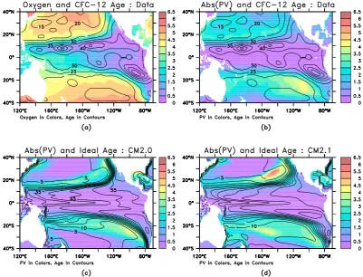
Fig. 1. Oxygen minimum zones, age and potential vorticity in models and data at 300 m in the Central Pacific. (a) Oxygen in ml/l from Conkright et al. (2002) (colors) and CFC-12 age in years (contours). CFC-12 age is computed from the dataset of (Willey et al., 2004) from the date at which the in-situ pCFC12 would have been in equilibrium with the atmosphere. The edge of the oxygen minimum zone occurs in a region of strong age gradients. Note also the asymmetry between the Northern and Southern zones. (b) Potential vorticity in s−3×10⁹ (f N2colors) and CFC-12 age (contours) for same region. The boundary of the old waters corresponds to a boundary between stratified interior waters (high PV) and weakly stratified waters in the shadow zone (low PV). (c) Potential vorticity (colors) and ideal age (contours) in model CM2.0, 67.5 years after the start of the 1990 control run. While ideal age is not directly comparable to CFC age, many of the same features are seen in the model as in the data. (d) Potential vorticity and ideal age in CM2.1 model 67.5 years after the start of the 1990 control run.
3 Results
The oxygen minimum zones reflect the underlying dynamics of the ocean circulation. At many depths and along many isopycnals, clear plumes of oxygen-rich water emanate from the eastern polar corners of the basins and seem to follow the gyre circulation into the interior. In the southeast Pacific, for example, Reid (1985) showed that the boundary between low oxygen and high oxygen zones at mid-depths corresponds to boundaries in steric height corresponding to boundaries be-tween flow rapidly ventilated from the south and more slug-gish closed circulations or even flow from the north.
The ventilated thermocline theory of Luyten et al. (1983, henceforth LPS) suggests that such a boundary should ex-ist as a result of potential vorticity (PV) dynamics. Be-cause eastern boundaries cannot provide the friction to allow parcels to change their potential vorticity f/H, geostrophic
flow right at the boundary will be sluggish. Instead boundary waves act to homogenize H, removing pressure gradients and resulting in north-south potential vorticity gradients which act to block the gyre flow. The resulting shadow zones have small values of PV which cannot connect directly to larger values found in outcrop regions of mode and intermediate waters. As a result, these regions cannot be directly venti-lated by time-mean geostrophic flows and will be older than the ventilated interior gyre. The LPS theory does not predict the age of the shadow zones, since the processes responsible (diapycnal and isopycnal mixing) are not included.
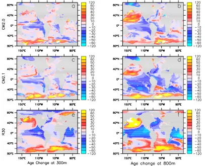
Fig. 2. Age changes under global warming (second century of 2×CO2 – 1860 control). Note that scale is linear from−60 to 60 years, with extreme age changes being shown by the most extreme colors. (a) CM2.0 at 300 m. (b) CM2.0 at 800 m. (c) CM2.1 at 300 m (d) CM2.1 at 800 m. (e) R30 at 300 m. (f) R30 at 800 m.
and potential vorticity (defined here asf N2wheref is the Coriolis parameter andNis the buoyancy frequency) as sug-gested by LPS. The coupled models (Figs. 1c, d) are able to reproduce the potential vorticity gradient, and have a signifi-cant gradient in ideal age at this point as well. Note that the CFC-12 age is not strictly comparable to the ideal age due to the fact that it will be biased high by lack of equilibration in sinking water (Russell and Dickson, 2003), and biased low by mixing. Qualitatively though, the CFC-12 ages range be-tween 35 and 50 years in the shadow zones, while the ideal age is around 45 years, suggesting that the ventilation in the models is roughly comparable to the observations.
In the western Pacific, there are clear differences between the models and the data. The data show a strong asymmetry between older, lower oxygen waters to the north and younger, higher oxygen waters to the south while the model produces a more symmetric pattern. This is because the model has equatorial winds that are much more symmetric about the Equator than in the real world. When the ocean model is forced with observed winds, there is a strong North
Equa-torial Counter Current and a weak South EquaEqua-torial Counter Current, in agreement with observations. This means that the old, low oxygen water in the east is much more efficiently transported to the west in the Northern Hemisphere relative to the Southern.
A. Gnanadesikan et al.: Ventilation under global warming 47
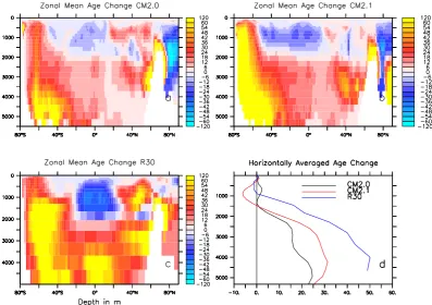
Fig. 3. Average changes in age under global warming (second century of 2×CO2 – 1860 Control). Note that scale is linear from−60 to 60 years, with extreme age changes being shown by the most extreme colors. (a) Zonally averaged change in CM2.0 (b) Zonally averaged change in CM2.1 (c) Zonally averaged change in R30 (d) Horizontal average in the three cases.
the extent to which Northern Indian Ocean becomes younger, with the R30 model suggesting that this region will become significantly younger at 300 m, the CM2.0 model showing it becoming older, while CM2.1 suggests a mixture of changes. All three models do show decreases in age in the shadow zones, particularly in the Pacific.
A few other regions also show consistent changes between the three models reported here. At 800 m, the Canada Basin becomes younger in all three models shown here, as well as in the simulation of (Bryan et al., 2006). Additionally, the western part of the Atlantic subtropical gyre also becomes younger. While neither of these regions shows the near-total drawdown in oxygen found in the oxygen minimum zones, both regions are places where the apparent oxygen utilization is relatively high.
The age decreases at intermediate depths contrast with age increases in the deep, as shown by zonally-averaged ideal age change in Fig. 3. All three models show the tropics becoming younger above depths of 2000 m, with larger increases be-low this depth. When horizontal averages are taken, it can be seen that the average increase in deep ideal age is between 20 and 50 years, with the largest values being found in the R30 model. At shallower depths, the age may actually decrease in the horizontal average, depending on whether the increase
in ideal age in the subpolar regions is sufficient to cancel out the decrease in ideal age in the tropics. Although the magni-tude of the age changes are much bigger in the R30 model, the broad similarity of the three patterns of ideal age change suggests that the basic pattern of change is not merely a func-tion of details such as whether the model is flux-adjusted or whether the model at equilibrium (in both cases the R30 model is while CM2 models are not). It is also worth noting that very similar changes have recently been reported in the NCAR CCSM3 model (Bryan et al., 2006).
Fig. 4. Volume of “young” water (with an ideal age less than 50 years) in the CM2 series. Solid lines are the 1860 control, dashed lines the doubled carbon dioxide run. (a) CM2.0. (b) CM2.1.
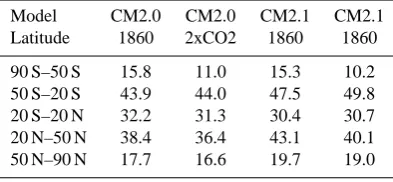
Table 1. Volumes of water (million cubic km) younger than 50 years old.
Model CM2.0 CM2.0 CM2.1 CM2.1 Latitude 1860 2xCO2 1860 1860
90 S–50 S 15.8 11.0 15.3 10.2 50 S–20 S 43.9 44.0 47.5 49.8 20 S–20 N 32.2 31.3 30.4 30.7 20 N–50 N 38.4 36.4 43.1 40.1 50 N–90 N 17.7 16.6 19.7 19.0
both models. However, the volume of young water in the mid-latitudes of the Southern Hemisphere actually increases under global warming in CM2.1 and holds essentially con-stant in CM2.0 (Table 1). Russell et al. (2006) argue that this increase can be attributed to the poleward shift of the South-ern Hemisphere westerly winds found under global warming. On short time scales most of the anthropogenic carbon taken up by the ocean ends up in these relatively young waters.
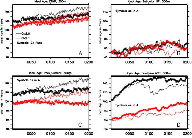
The changes in the shadow zones are particularly inter-esting because they occur in regions where the variability in ideal age is relatively low. Figure 5 shows time series of ideal age at 300 m in four regions, the Eastern Tropical North Pacific (5 N–15 N, 150 W–90 W) which includes the core of the northern shadow zone, the subpolar North Pacific (45 N– 55 N, 150 E–150 W), a region including the Peru Current and offshore waters (10 S–25 S, 100 W–70 W) and the southern ocean (65 S–55 S). Note that CM2.1 is younger than CM2.0 at this depth throughout the world ocean, reflecting in part the difference in the initial spinup. All the control simula-tions show clear trends in the early, and in some cases the later part of the record as well, reflecting the spinup of the age field. In the two shadow zone regions, there is a very clear separation between the global warming cases and the control cases, with the variability occurring on very short time scales (2–5 years) and much smaller than the signal. At or near the
time of CO2 doubling the shadow zones have begun to be-come clearly younger. By contrast in the subpolar regions, the variability is of the same order of magnitude as the net change.
This result has interesting implications for where we should look for the impact of climate change. Doubling carbon dioxide alone corresponds to a radiative forcing of 3.7 W/m2. This is only about 25% larger than the 2.8 W/m2 that is seen today in our models (T. Knutson, personal com-munication). Thus, our results suggest that significant and detectable changes in shadow zone ventilation may be oc-curring today.
4 Discussion
In order to understand the results of the coupled model, it is necessary to distinguish between two conceptual models of the ideal age. The first may be thought of as a “pipe” model, in which the age at a point simply reflects the time required for water to reach that point from a surface outcrop. In such a picture a reduction of the advective or diffusive transport would result in an increase in the age. However, one can propose an alternative “network” model in which there are many different pathways to reach the same point. In such a model the age is actually the centroid of a spectrum of ages, reflecting many different pathways by which surface waters can reach a particular point (see Khatiawala et al., 2001, for a more detailed discussion of this issue). The age at a point can then change not only as the time associated with each path-way changes, but as the relative proportion of waters taking separate pathways changes.
A. Gnanadesikan et al.: Ventilation under global warming 49
Fig. 5. Time series of the ideal age at 300 m in the CM2 series. Black lines are for CM2.0, red for CM2.1. Lines with symbols are the doubled CO2run. (A) Eastern Tropical North Pacific. Note that the ages under global warming begin to diverge about year 50. (B) Subpolar North
Pacific. Note substantial decadal variability of same order of magnitude as climate change. (C) Peru Current. Here the difference between the ages cannot be attributed to spinup alone, as year 80 of the control CM2.1 is still substantially younger than CM2.0. (D) Southern Ocean. The same difference in age is attributable to a difference in ventilation forced by the higher Southern Ocean winds.
formation of bottom water, which flows from polar regions into the tropics and upwells into the interior, aging as it does so. The other involves the diffusion of tropical surface water from above (which, in models such as the HILDA code of Shaffer and Sarmiento, 1995, is taken as a representation of the wind-driven gyre circulation as well as explicit diapycnal diffusion). The equations governing age in the model interior is then
∂A
∂t =1−w
∂A
∂z +
∂ ∂zKv
∂A
∂z (1)
wherew is the upwelling velocity andKvis a vertical
dif-fusion coefficient. Thus the natural rate of change of age is one year per year (first term on the right-hand side of Eq. 1) but this can be altered by the advection or diffusion of age from above or below. At steady-state, this equation can be rearranged as
w∂A
∂z −
∂ ∂zKv
∂A
∂z =1 (2)
A simple solution can be derived by setting A=0 at the boundaries of the model interior which we define as
z=0,−D. While models such as the HILDA code allow for lateral exchange with a well-mixed polar deep box and in-ject the deep water from this box, such additional complexity does not add additional insight relative to the simple condi-tion of fixing the bottom water and top at an age of 0. With these boundary conditions and an initial condition ofA=0
everywhere, Eq. (1) will initially be dominated by the time rate of change and will age at approximately one year per year, except near the top boundary, where there will be a dif-fusive flux of young water from above and the bottom bound-ary, where there will be both an advective and diffusive flux of young water from below. Over time, these boundary fluxes will penetrate further and further into the interior, resulting in a steady-state solution given by Eq. (2), the solution to which is
A= 1
w
z+D(1−e
zw/Kv)
1−e−wD/Kv
(3) which depends critically on the Peclet numberP e=wD/Kv.
0 500 1000 1500 2000 2500 −4000
−3000 −2000 −1000 0
1D model of Ideal Age, Kv=0.1
Solid: Mu=36 Sv Pe=40 Dashed: Mu=18 Sv Pe=20
A
Age in Years
Depth in m
0 500 1000
−4000 −3000 −2000 −1000 0
1D model of Ideal Age, Kv=1
Solid: Mu=36 Sv Pe=4 Dashed: Mu=18 Sv Pe=2
B
Age in Years
Depth in m
0 500 1000 1500 2000 −4000
−3000 −2000 −1000 0
Age Change (Reduced Upwelling) Kv=0.1
C
Age in Years
Depth in m
−50 0 50 100 150 −4000
−3000 −2000 −1000 0
Age Change (Reduced Upwelling) Kv=1
D
Age in Years
Depth in m
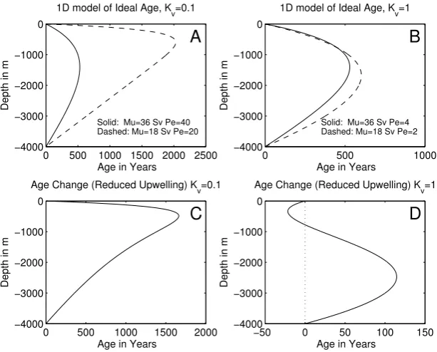
Fig. 6. Solutions generated by a one-dimensional advective-diffusive model of ideal age. In left-hand column, solutions are shown for
P e=wD/Kv=40, 20 (w=0.5,1×10−7m/s corresponding to 18 and 36 Sv of upwelling andKv=10−5m2/s=0.1 cm2/s). In right hand column
solutions are shown for lower values ofP e=(4,2) corresponding to the same pair of upwelling values and a higher diffusive coefficient of 1 cm2/s. The top row shows the equilibrium solutions, the bottom row the difference between these solutions.
Fig. 7. Budget of age in CM2.1 models. The terms are scaled relative to the volume of the ocean, so that a flux of 1 would mean that the flux was accounting for all of the aging in the ocean below the surface layer. (a) Advective age flux, showing a significant decrease in the advective flux under global warming. (b) Diffusive age flux (convection+implicit vertical diffusion + isopycnal mixing and advection) showing a relatively small change in this flux. (c) Flux changes under global warming. Decrease in advective flux dominates, accounting for the modelled decrease in age above 2000 m and the modelled increase in age below that point.
Such a picture is supported by Fig. 7, which shows the horizontally integrated budget of ideal age from years 220 to 240 of the 2X and 1860 control runs. The diffusive transport of age (encompassing vertical diffusion, convection, and the vertical transport associated with eddies) hardly changes at
A. Gnanadesikan et al.: Ventilation under global warming 51
Fig. 8. Overturning change under global warming associated with the three models. Contour interval is every 2 Sv, while colors change every 4 Sv. (a) CM2.0. (b) CM2.1 (c) R30.
in all three models. As a result the age in the intermediate waters drops (less old water is being injected from below) and that at depth increases (less old water is being exported vertically). This explains in part why the signature of global warming on ideal age is so much larger in the R30 model. In the R30 model (which is at equilibrium) ideal ages in the deep ocean are very high. Reducing the upwelling of this old water produces a much bigger signal than in the CM2 series. An additional reason for the difference between the models is that the magnitude of the overturning changes dif-fers between the models. The CM2.0 model has very little deep convection in the Southern Ocean (Gnanadesikan et al., 2006) and little formation of Labrador Sea Water. As a result, when the planet warms and these regions restratify the over-turning changes relatively little. By contrast, in CM2.1, the Labrador Sea actually cools under global warming as con-vection in this region shuts off (Stouffer et al., 2006). The R30 model has an even larger decrease in the overturning, further enhancing the increase in age at depth and decrease at age in the intermediate waters.
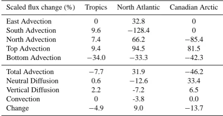
More detailed examination of the budget reinforces the idea that changes in the relative contributions of water masses are important for driving changes in age. The total age budget for the tropics is shown in first column of Table 2, where changes in the age supply due to various processes are scaled by the age source over the region. The dominant term is clearly a reduction in the advection of old water through the bottom (all other terms in this column tend to increase the age in this region). Thus, even though the edge of the shadow zone appears to be simulated in terms of a potential vorticity front (as suggested by a theory that assumes an adi-abatic interior), diapycnal fluxes still play an important role in setting the exact value of the age within the shadow zone. The age budgets for other regions where the ocean be-comes younger also show the effects of changing the mix of source waters. For example in the North Atlantic (second column of Table 2) the largest decrease is seen in the
ad-Table 2. Changes in age flux into various regions that show waters becoming younger under global warming in CM2.1 model. Values are scaled by the age source within the volume, so that a change of−35 means that the age fluxes would compensate 35% of the local aging. First column is the tropics between depths of 285 m and 1270 m. Second is the west central North Atlantic (between 18 N and 44 N, west 35 W and between 416 m and 1270 m). Third column is the Canadian Arctic between 416 m and 1270 m south of the model grid latitude of 80 N.
Scaled flux change (%) Tropics North Atlantic Canadian Arctic
East Advection 0 32.8 0
South Advection 9.6 −128.4 0
North Advection 7.4 66.2 −85.4
Top Advection 9.4 94.5 81.5
Bottom Advection −34.0 −33.3 −42.3
Total Advection −7.7 31.9 −46.2
Neutral Diffusion 0.6 −12.6 33.4
Vertical Diffusion 2.2 -7.2 6.5
Convection 0 -3.8 0.0
Change −4.9 9.0 −13.7
0.904
1.452
−0.039
0.152
0.026 −0.116
Phosphate (Tmol/yr) 220m
1131m
30S 30N
−0.600
−0.29
−1.490
Advection
Diffusion
Biological source/sink
220m
1131m
30S 30N
Oxygen (Tmol/yr)
−198.8
120.4 −9.6
54.7 11.7 3.2
67.2
16.3
−65.2
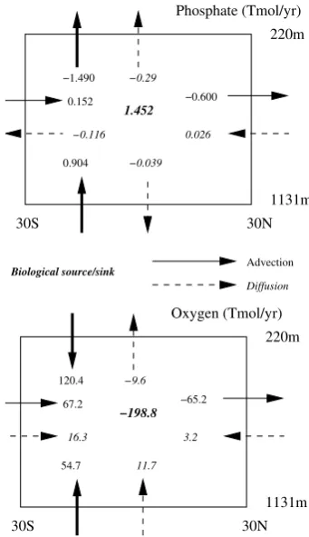
Fig. 9. Budgets of phosphate (top) and oxygen (bottom) in the 220– 1131 m depth range from 30 S to 30 N in the PRINCE2A model of Gnanadesikan et al. (2004). Solid lines are advective fluxes, dashed lines mixing fluxes. The italicized bold numbers indicate biological sources or sinks. Upwelling from below 1100 m supplies a signifi-cant amount of phosphate and oxygen to this region.
5 Conclusions
We have shown that under global warming, a number of re-gions that are relatively poorly ventilated at the present may actually become more tightly coupled to the surface. This is because the relative mix of waters entering these regions may change. This effect is particularly prominent in the oceanic shadow zones where multiple models (our three in addition to the model of Bryan et al., 2006), differing significantly in how atmospheric and oceanic processes are represented all show the ideal age declining. Is it possible to isolate what effect such changes might have on oxygen and nutrient cy-cles? How important is this deep upwelling for maintaining tropical production, and what is its effect on deep oxygen?
As we do not have access to an earth system model in which all of the relevant terms have been saved, we are forced to approach these questions by looking at the role of deep up-welling fluxes in coarse diagnostic ocean models. We use the 4-degree, 24 level, PRINCE2 model reported in Gnanade-sikan et al. (2004) to obtain a rough estimate of the
impor-tance of the deep upwelling and mixing fluxes for the oxy-gen and phosphorus cycles. As described in Gnanadesikan et al. (2004) this model produces reasonable simulations of temperature, salinity, oxygen, phosphorus, radiocarbon, and particle export when compared with data. Figure 9 shows the budget of oxygen and phosphorus between 30 S and 30 N and 220–1130 m in this model. Advective fluxes are shown with solid arrows, diffusive fluxes with dashed arrows and biological sources and sinks with italicized bold numbers. Note that the vertical fluxes are not necessarily due to di-apycnal processes, isopycnal flows which exchange oxygen-rich and phosphate-poor surface water with oxygen-poor and phosphate-rich intermediate water effectively transport oxy-gen in the vertical. As can be seen in the bottom panel of Fig. 9 the upwelling of deep waters acts as an important source of oxygen for the intermediate depths, accounting for approximately 36% of the total oxygen demand. The up-welling also serves as a source of phosphate to the region, equivalent to 60% of the phosphate source. This implies that a slowdown in the circulation would reduce mid-depth phos-phate concentrations (and thus presumably the biological cy-cling of phosphate within the tropics) by a larger fraction than it would decrease oxygen. Circulation changes brought on by global warming might, therefore, lead to an increase in mid-depth oxygen, countering some fraction of the decrease which would be caused by decreased oxygen solubility asso-ciated with warming. Further investigation of this, however, will have to await detailed analysis of term budgets in full Earth System Models.
In summary, we have shown that global warming changes the balance of waters feeding the intermediate layers, in-creasing the fraction of younger surface waters and decreas-ing the fraction of older deep waters. The results of this change are likely to be particularly complex in tropical oxy-gen minimum zones, where old deep waters serve as a source of oxygen and nutrients to the subtropical ocean.
Acknowledgements. The authors thank the Geophysical Fluid Dynamics Laboratory for support of this research, W. Cooke and R. Slater for their work on including ideal age in the models, and T. Delworth for sharing the results of the R30 run. Comments from K. Rodgers, E. Galbraith, two anonymous reviewers and B. Barnier are gratefully acknowledged.
Edited by: B. Barnier
References
Altabet, M. A., Murray, D. W., and Prell, W. L.: Climatically linked oscillations in Arabian Sea denitrification over the past 1 m.y.: Implications for the marine nitrogen cycle, Paleoceanography, 14, 732–743, 1999.
A. Gnanadesikan et al.: Ventilation under global warming 53
Conkright, M. E., Antonov, J. I., Baranova, O., Boyer, T. P., Gar-cia, H. E., Gelfeld, R., Johnson, D. D., Locarnini, R. A., Mur-phy, P. P., O’Brien, T. D., Smolyar, I., and Stephens, C.: World Ocean Database 2001, Volume 1: Introduction, edited by: Lev-itus, S., NOAA Atlas, NESDIS 42, U.S. Government Printing Office, Washington, D.C., 167 pp, 2002.
Delworth, T. L., Stouffer, R. J., Dixon, K. W., Spelman, M. J., Knut-son, T. R., Broccoli, A. J., Kushner, P. J., and Wetherald, R. T.: Review of simulations of climate variability and change with the GFDL R30 coupled climate model, Clim. Dyn., 19(7), 555–574, 2002.
Delworth, T., Broccoli, A. J., Rosati, A., et al.: GFDL’s global cou-pled climate models- Part 1: Equilibrium simulations, J. Climate, 18, 643–674, 2006.
Elkins, J. W., Wofsy, S. C., McElroy, M. C., Kolb, C. E., and Ka-plan, W. E.: Aquatic sources and sinks for nitrous oxide, Nature, 275, 602–606, 1978.
Galbraith, E. D., Kienast, M., Pedersen, T. F., and Calvert, S. E.: Glacial-interglacial modulation of the marine nitrogen cycle by high-latitude O2 supply to the global thermocline, Paleoceanog-raphy, 19, PA4007, doi:10.1029/2003PA001000, 2004.
Gent, P. and McWilliams, J. C.: Isopycnal mixing in ocean circula-tion models, J. Phys. Oceanogr., 20, 150–155, 1990.
The GFDL Global Atmospheric Model Development Team: The new GFDL global atmosphere and land model AM2-LM2: Eval-uation with prescribed SST simulations, J. Climate, 17(24), 4641–4673, 2004.
Gnanadesikan, A., Dunne, J. P., Key, R. M., Matsumoto, K., Sarmiento, J. L., Slater, R. D., and Swathi, P. S.: Oceanic ven-tilation and biogeochemical cycling: Understanding the phys-ical mechanisms that produce realistic distributions of tracers and productivity, Global Biogeochem. Cycles, 18, GB4010, doi:10.1029/2003GB002097, 2004.
Gnanadesikan, A., Dixon, K. W., Griffies, S. M., et al.: GFDL’s global coupled climate models- Part 2: The baseline ocean sim-ulation, J. Climate, 18, 675–697, 2006.
Griffies, S. M., Gnanadesikan, A., Dixon, K. W., Dunne, J. P., Gerdes, R., Harrison, M. J., Rosati, A., Russell, J. L., Samuels, B. L., Spelman, M. J., Winton, M., and Zhang, R.: Formulation of an ocean model for global climate simulations, Ocean Sci., 1, 45–79, 2005,
http://www.ocean-sci.net/1/45/2005/.
Griffies, S. M., Harrison, M. J., Pacanowski, R. C., and Rosati, A.: A Technical Guide to MOM4. GFDL Ocean Group Technical Report No. 5, Princeton, NJ: NOAA/Geophysical Fluid Dynam-ics Laboratory, 2003.
Gruber, N. and Sarmiento, J. L.: Global patterns of marine nitro-gen fixation and denitrification, Global Biogeochem. Cycles, 11, 235–266, 1997.
Hirst, A. C., Gordon, H. D., and O’Farrell, S. P.: Global warm-ing in a coupled climate model includwarm-ing oceanic eddy-induced advection, Geophys. Res. Lett., 21, 3361–3364, 1996.
Lin, S.-J.: A “vertically Lagrangian” finite-volume dynamical core for global models, Mon. Wea. Rev., 132(10), 2293–2307, 2004. Lionello, P. and Pedlosky, J.: The role of a finite density jump at the
bottom of the quasi-continuous ventilated thermocline, J. Phys. Oceanogr., 30, 338–351, 2000.
Luyten, J. L., Pedlosky, J., and Stommel, H. M.: The ventilated thermocline, J. Phys. Oceanogr., 13, 292–309, 1983.
Manabe, S. and Stouffer, R. J.: Multiple-century response of a cou-pled ocean- atmosphere model to an increase of atmospheric car-bon dioxide, J. Climate, 7, 5–23, 1994.
Pacanowski, R., Dixon, K., and Rosati, A.: The GFDL Modular Ocean Model users guide version 1, GFDL Ocean Group Tech Rep 2, pp. 44, 1991.
Reid, J. L.: On the total geostrophic circulation of the South Pacific: Flow patterns, tracers and transports, Progress in Oceanography, 16, 1–61, 1985.
Russell, J. L. and Dickson, A. G.: Variability in oxygen and nu-trients in South Pacific Antarctic Intermediate Water, Global Biogeochem. Cycles, 17(2), 1033, doi:10.1029/2000GB001317, 2003.
Russell, J. L., Dixon, K. W., Gnanadesikan, A., Stouffer, R. J., and Toggweiler, J. R.: Southern Ocean Westerlies in a warm-ing world: Proppwarm-ing open the door to the deep ocean, J. Climate, 19, 6382–6390, 2006.
Sarmiento, J. L., Hughes, T. M. C., Stouffer, R. J., and Manabe, S.: Simulated response of the ocean carbon cycle to anthropogenic climate warming, Nature, 393, 245–249, 1998.
Sarmiento, J. L., Slater, R., Barber, R., Bopp, L., Doney, S. C., Hirst, A. C., Kleypas, J., Matear, R., Mikolajewicz, U., Monfray, P., Soldatov, V., Spall, S. A., and Stouffer, R. J.: Response of ocean ecosystems to global warming, Global Biogeochem. Cy-cles, 18, GB3003, doi:10.1029/2003GB002134, 2004.
Stouffer, R. J., Weaver, A. J., and Eby, M.: A method for obtaining pre-twentieth century initial conditions for use in climate change studies, Clim. Dyn., 23, 327–339, 2004.
Stouffer, R. J., Broccoli, A. J., Delworth, T. L., Dixon, K. W., Gudgel, R., Held, I., Hemler, R., Knutson, T., Lee, H.-C., Schwartzkopf, M. D., Soden, B., Spelman, M. J., Winton, M., and Zeng, F.: GFDL’s CM2 Global Coupled Climate Models – Part 4: Idealized Climate Response, J. Climate, 19, 723–740, 2006.
Vecchi, G. A. and Soden, B. J.: Global warming and the weakening of the tropical circulation, J. Climate, in press, 2007.
Vecchi, G. A., Soden, B. J., Wittenberg, A. T., Held, I. M., Leet-maa, A., and Harrison, M. J.: Weakening of tropical Pacific atmospheric circulation due to anthropogenic forcing, Nature, 441(7089), 73–76, 2006.
Volk, T. and Hoffert, M. J.: Ocean carbon pumps: analysis of rela-tive strengths and efficiencies in ocean-driven atsmopheric pCO2 change, in: The Carbon Cycle and Atmospheric CO2:
Natu-ral variations Archean to Present, edited by: Sundquist, E. and Broecker, W. S., Geophys. Monogr. Ser., 32, 163–184, 1985. Wallmann, K.: Feedbacks between oceanic redox states and
marine productivity:A model perspective focused on benthic phosphorus cycling, Global Biogeochem. Cycles, 17, 1084, doi:10.1029GB001968, 2003.
Washington, W. M. and Meehl, G. A.: Climate sensitivity due to in-creased CO2: experiments with a coupled atmosphere and ocean general circulation model, Clim. Dyn., 4, 1–38, 1989.