Nonlinear Processes
in Geophysics
c
European Geophysical Society 2002
Two-dimensional MHD model of the reconnection diffusion region
N. V. Erkaev1, V. S. Semenov2, and H. K. Biernat3
1Institute of Computational Modelling, Russian Academy of Sciences, Krasnoyarsk, 660036, Russia 2Institute of Physics, University of St. Petersburg, St. Petergof, 198504, Russia
3Space Research Institute, Austrian Academy of Sciences, Schmiedlstrasse 6, Graz, A-8042, Austria Received: 06 August 2001 – Accepted: 16 October 2001
Abstract. Magnetic reconnection is an important process
providing a fast conversion of magnetic energy into thermal and kinetic plasma energy. In this concern, a key problem is that of the resistive diffusion region where the reconnec-tion process is initiated. In this paper, the diffusion region is associated with a nonuniform conductivity localized to a small region. The nonsteady resistive incompressible MHD equations are solved numerically for the case of symmetric reconnection of antiparallel magnetic fields. A Petschek type steady-state solution is obtained as a result of time relax-ation of the reconnection layer structure from an arbitrary initial stage. The structure of the diffusion region is studied for various ratios of maximum and minimum values of the plasma resistivity. The effective length of the diffusion re-gion and the reconnection rate are determined as functions of the length scale and the maximum of the resistivity. For suf-ficiently small length scale of the resistivity, the reconnection rate is shown to be consistent with Petschek’s formula. By increasing the resistivity length scale and decreasing the re-sistivity maximum, the reconnection layer tends to be wider, and correspondingly, the reconnection rate tends to be more consistent with that of the Parker-Sweet regime.
1 Introduction
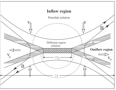
Magnetic reconnection is a physical process in plasmas pro-viding a disruption of current layers and a fast conversion of magnetic energy into another kinds of energy, such as bulk motion of the plasma, heating, and acceleration of parti-cles. This process is considered to be very important in solar, space, and laboratory plasmas (Hones, 1984; Priest, 1985). In the model proposed by Petschek (1964), the whole recon-nection area consists of large convective and small diffusion regions (Fig. 1). In the convective region, plasma is accel-erated at the slow shock fronts which originate from a small Correspondence to: H. K. Biernat
diffusion region. The intensity of the reconnection process is characterized by the reconnection rate which is determined by the electric field generated in the diffusion region. There-fore, the diffusion region is a central subject concerning the reconnection problem. An alternative model is that of Sweet (1958) and Parker (1957) who consider magnetic reconnec-tion as a pure diffusive process.
Laboratory experiments of magnetic reconnection (Ji et al., 1999), as well as numerical simulations carried out by Biskamp (1986) and Scholer (1989) for a constant resistivity are in favor of the Sweet–Parker solution. On the other hand, in cases of nonuniform resistivity localized to a small region, the numerical simulations (Scholer, 1989; Ugai, 1999) show the evidence of Petschek–type reconnection with plasma ac-celeration at the shock fronts.
For the convective region, an analytical solution of the ideal MHD equations can be obtained as an asymptotic se-ries in the reconnection rate which is considered to be a small parameter. For the diffusion region, it seems to be impossi-ble to find an analytical solution, and hence a solution has to be obtained numerically (Erkaev et al., 2000). The re-connection rate can be determined by matching the solutions corresponding to the diffusion and convective regions.
The aim of our paper is to study a numerical MHD model of the diffusion region for a nonuniform conductivity, and to obtain the reconnection electric field and the reconnection rate as functions of the amplitude and length scale of the re-sistivity.
Fig. 1. The Petschek reconnection model: the outer convective and the inner diffusion regions.
2 MHD equations. Petschek solution
In our model, the plasma is governed by the resistive steady– state MHD system of equations (Landau and Lifshitz, 1984)
(ρv· ∇)v= −∇P + 1
4π(B· ∇)B, (1)
E+1
c(v×B)= c
4π σ (x, y)curlB, (2)
divB=0, divv=0, (3)
where incompressibility is assumed; quantityP is the total pressure.
Outside of the diffusion region, dissipation is not impor-tant, and we can use the ideal system of MHD equations.
In an incompressible plasma the following relations have to be satisfied at the shock front
{Bn} =0, (4)
{vn} =0, (5)
{P} =0, (6)
1
4πBnBt−ρvnvt
=0, (7)
{Bnvt−vnBt} =0, (8)
where the subscriptsnandtdenote components normal and tangential to the shock front.
Within two dimensions, in Cartesian coordinatesx, y (x
is directed along the current sheet), the Petschek solution, which is valid in the convection region, can be presented in a simple analytical form (Petschek, 1964; Vasyliunas, 1975).
Inflow region:
vx=0, vy= −εVA, (9)
Bx=B0− 4εB0
π ln L
p
x2+y2,
By = 4εB0
π arctan x
y. (10)
Outflow region:
vx=VA, vy=0, Bx=0, By=εB0. (11) The shock front in the first quadrant is described by a linear function
y=εx. (12)
Just upstream of the shock, the normal magnetic field com-ponent is
By=2εB0. (13)
The reconnection rate is defined as
ε=E0/EA<<1, (14) where ε is supposed to be a small parameter in the prob-lem. HereE0is the electric field which is constant in the 2D model, andEA = 1cVAB0is the Alfv´en electric field, based onVA=B0/(4πρ0)1/2andB0.
Expressions (9)–(13) are asymptotic solutions with respect toε(zero and first order terms in the inflow region and only zero order terms in the outflow region) of the ideal MHD system of Eqs. (1)–(3) and the Rankine–Hugoniot shock re-lations (4)–(8).
Petschek did not obtain a solution for the diffusion region; instead, he suggested an upper estimation for reconnection rate asε∼1/lnRemwhich is based on some simple physi-cal ideas. Generally speaking, this implies that the Petschek model gives any reconnection rate from the Sweet–Parker value 1/√Rem up to 1/lnRem, and for a long time, it was unclear whether Petschek reconnection could be faster than Sweet–Parker reconnection. This problem can be solved by matching a solution for the diffusion region and the Petschek solution ((9)–(13).
3 Diffusion region scaling
To obtain the boundary layer MHD equations suitable for the diffusion region, we normalize the MHD parameters to the quantities taken at the upper boundary of the diffusion region
˜
Rem=4π σ∗VAdlc/c2, x˜ =x/ lc, ˜
y =y/ lc q
˜
Rem, B˜x=Bx/Bd,
˜
By=By/Bd q
˜
Rem, V˜x =Vx/VAd,
˜
Vy=Vy/VAd q
˜
Rem,
˜
Ed=Ezc/(BdVAd) q
˜
Rem. (15)
Hereσ∗is the minimal conductivity and quantitylcis the length scale of the conductivity. Subscript “d ” denotes pa-rameters taken at the upper diffusion region boundary for
is equal to the normalized electric fieldE˜
d. This scaling for the diffusion region is similar to that for the Prandtl viscous layer (Landau and Lifschitz, 1984) and corresponds exactly to the Sweet–Parker case.
Considering 1/Re˜ m as a small parameter, we obtain the boundary layer equations
∂ ∂t(
˜
Vx)+ ˜Vx
∂ ∂x˜(
˜
Vx)+ ˜Vy
∂ ∂y˜(
˜
Vx)
− ˜Bx
∂ ∂x˜(
˜
Bx)− ˜By
∂ ∂y˜(
˜
Bx)= −
∂ ∂x˜(
˜
P ), (16)
∂ ∂y˜(
˜
P )=0, (17)
∂ ∂t ˜ Bx = ∂
∂y˜
˜
VxB˜y− ˜VyB˜x
+ ∂
∂y˜
η(x,˜ y)˜ ∂
∂y˜ ˜ Bx , (18) ∂ ∂t ˜ By = − ∂
∂x˜
˜
VxB˜y− ˜VyB˜x
− ∂
∂x˜
η(x,˜ y)˜ ∂
∂y˜
˜
Bx
, (19)
divB˜ =0, (20)
divv˜=0, (21)
whereη(˜ x,˜ y)˜ is the normalized resistivity of the plasma with the maximum value to be 1. It can be seen from Eq. (17) that the total pressure is constant across the diffusion region. This is a general feature of a boundary layer approximation.
4 Initial and boundary conditions. Numerical scheme
Starting with an initial MHD configuration under fixed boundary conditions, the time–dependent MHD solution converges to a steady state. The normalized total pressure is chosen to be 1. The internal reconnection rateε˜ is to be determined from the numerical solution as a result of time relaxation.
The distribution of the resistivity is traditional (Scholer, 1989; Ugai, 1999)
η(x,˜ y)˜ =de(−sxx˜2−syy˜2)+f, (22)
withd+f =1.
As the initial configuration, we choose a current sheet with a linear profile of the magnetic fieldB˜x =y,B˜y =0. The velocity components are assumed to be equal to zero at the initial moment,V˜x=0,V˜y=0.
At the upper (inflow) boundary, the tangential magnetic field component is assumed to be constant,B˜x =1, and the tangential velocity component vanishes, V˜x = 0. At the left boundary we have the symmetry conditions∂(B˜x)/∂x= 0, B˜y =0, V˜x =0.At the right boundary we keep free conditions suitable for a uniform flow in the outflow region
∂(B˜y)/∂x = 0, ∂(V˜y)/∂x = 0. At the lower boundary (y = 0) there is the symmetry condition for the tangential
magnetic field component,B˜
x = 0, and the non–flow con-dition for the normal velocity component,V˜
y = 0. At this boundary, the normal component of the magnetic fieldB˜yis obtained from the induction Eq. (19) on the liney=0,
∂ ∂t(
˜
By)+
∂ ∂x(
˜
VxB˜y)=
∂
∂x(ηJz), (23)
whereJz = ˜Re−m1∂B˜y/∂x−∂B˜x/∂y˜. The term∼ ˜Rem−1is included to stabilize the numerical scheme for the unsteady system of the boundary layer MHD equations.
To solve the MHD system numerically, we use a two step conservative finite difference numerical scheme with a rect-angular grid 145×100 in the first quadrant. From each time level (n), we calculate the parameters on the next time level
(n+1)in two steps. In the first step(n+1/2), diffusion is switched off, and we calculate the parameters for the in-termediate time level(n+1/2)using the equations in char-acteristic form. This is similar to the approach used in the Godunov method (Godunov and Ryabenkii, 1987). In the second step, we calculate the parameters for the next time level(n+1)using the equations in conservative form and tak-ing into account the diffusion terms approximated in implicit form. The details of the numerical algorithm are the follow-ing. TheB˜x component is found from thex-component of the induction equation
(B˜xi,kn+1− ˜Bxi,kn )/τ+
Gni,k++1/21/2−Gni,k+−1/21/2
/ hx =
∂/∂y˜
η(Bx/∂y˜− ˜Rem−1∂B˜y/∂x)˜ n+1
i,k
, (24) where quantities
Gni,k++1/21/2=
˜
BxV˜y− ˜VxB˜y n+1/2
i,k+1/2
(25) are determined by the method of characteristics at the time leveln+1/2.
The normal magnetic field component B˜y is determined from equation divB=0 approximated on a rectangular grid. The velocity componentV˜xis found from thex–component of the momentum Eq. (16),
(V˜xn+1− ˜Vxn)i,k/τ +
Qyi,k+1/2−Qyi,k−1/2 n+1/2
/ hy
+
Qxi+1/2,k−Qyi−1/2,k n+1/2
/ hx =0, (26) where
Qnyi,k+1/2+1/2=
˜
VxV˜y− ˜BxB˜y n+1/2
i,k+1/2
,
Qnxi++1/21/2,k =
˜
Vx2− ˜Bx2
n+1/2 i+1/2,k
. (27)
0
5
10
0 5
100 0.2 0.4 0.6 0.8 1
X Vx,sx=1, sy=1,d=0.95,f=0.05
Y
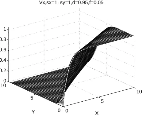
Fig. 2. Tangential velocity component.
0
5
10
0 5
10 −0.8 −0.6 −0.4 −0.2 0
X Vy,sx=1, sy=1,d=0.95,f=0.05
Y
Fig. 3. Normal velocity component.
5 Results of the numerical simulation
To estimate the convergence of the time–dependent solution to a steady state for eachn–th time step, we use the following criteria: max(|Vxn−Vxn−1|)/(1t|Vxmaxn |) <10−6.
For the case of localized resistivity, the system reaches the Petschek steady state with clear asymptotic behaviour (see Figs. 2–7): Vx → 1 in the outflow region;Vy → ˜εat the inflow boundary;Bxdecreases from 1 to 0 at the shock tran-sition;By→ ˜εin the outflow region; andBy →2ε˜from the inflow side of the shock (compare with the Petschek solution (9 – 12)).
In the 2D steady state, the total (convective plus dissipa-tive) electric field must be constant. The convective and to-tal electric fields obtained in our calculations are shown in Figs. 6 and 7. One can see that the total electric field is nearly constant except for small perturbations localized to the
out-0
5
10
0 5
100 0.2 0.4 0.6 0.8 1
X Bx,sx=1, sy=1,d=0.95,f=0.05
Y
Fig. 4. Tangential magnetic field component.
0
5
10
0 5
100 0.4 0.8 1.2
X By,sx=1, sy=1,d=0.95,f=0.05
Y
Fig. 5. Normal magnetic field component.
flow boundary due to some influence from the right-hand side boundary conditions.
The magnetic field lines and plasma flow steam lines are shown in Fig. 8. Here, the inflow and outflow regions are clearly separated by the slow shock wave originating from the central part of the diffusion region.
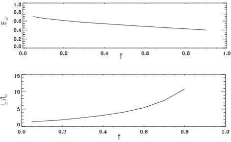
There is a well pronounced slow shock, as can be seen in the behaviour of all MHD parameters. The diffusion region reconnection rate is equal to the normalized diffusion region electric fieldE˜d which is obtained to be in the range 0.4 <
˜
Ed<0.7, as shown in Fig. 9 (top).
resis-0
5
10
0 5
10 −1 −0.8 −0.6 −0.4 −0.2 0
X Ezcon=v×B,sx=1, sy=1,d=0.95,f=0.05
Y
Fig. 6. Convective electric field−(v×B)z.
0
5
10
0 5
10 −1 −0.8 −0.6 −0.4 −0.2 0
X Ez,sx=1, sy=1,d=0.95,f=0.05
Y
Fig. 7. Total electric field in the diffusion region.
tivity of the plasma is localized to a small region, whereas for constant resistivity, the Sweet–Parker regime is realized (Erkaev et al., 2000).
Figure 9 shows the normalized diffusion region electric field (top) and length scale (bottom) as functions of the pa-rameterf. This parameter is introduced as the ratio of the background resistivity to the maximum of the resistivity, and it varies in the range from 0 to 1. The value 1 corresponds to the case of uniform resistivity.
The length of the diffusion region ld, as defined above, is the size of the region where the convective electric field
E = −v×B/c(which is zero at the origin) reaches some level close to the asymptotic value (say 0.9). For the case of localized resistivity, quantityldpractically coincides with the scale of the inhomogeneity of the conductivity when the maximum of the resistivity is much larger than the back-ground resistivity.
0 2 4 6 8 10
0 2 4 6 8 0
Fig. 8. Magnetic field lines and plasma flow stream lines.
f l/d
lc Ed
f
Fig. 9. Electric field and length scale of the diffusion region as functions of the amplitude of conductivity variation.
6 Reconnection rate
To find the reconnection rate, we have to determine the mag-netic field at the boundary of the diffusion region Bd (for details, see Appendix)
Bd =B0
1−4ε
π ln L ld
. (28)
The electric field must be constant in the whole inflow re-gion, hence
vydBd=v0B0, (29)
0Bd2=εB02, (30) where the reconnection rates are defined as
0=vd/VAd, ε=v0/VA0.
Using the relation0= ˜(Re˜ m)−1/2we obtain ˜
Bd3/2=εB 3/2 0
p
G(K)
0 1 2 3 4 5
0.02 0.04 0.06 0.08
K
e
1
2
L / l , 2 10d
4
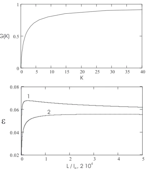
Fig. 10. FunctionG(K)and the reconnection rate as a function of the ratioL/ ld. Curves 1, 2 correspond to Reynolds numbers 104
and 105, respectively.
SubstitutingBd from Eq. (28), we determine finally the fol-lowing equation for the reconnection rateε
˜
1−4ε
π ln L ld
3/2
=εpRem l
c
L
1/2
, (32) where Rem is defined as the magnetic Reynolds num-ber for the global scale and the minimal conductivity,
Rem =4π σ∗VAL/c2. Here, the internal normalized recon-nection rate˜is obtained from the numerical solution of the diffusion region problem (see Fig. 9), 0.7> >˜ 0.4
An important parameter for the reconnection rate is
K=4 ln(L/ ld)
π√Rem
L
lc 1/2
.
The reconnection rate can be expressed through the function
G(K),
ε= π 4
1 ln(L/ ld)
G(K), (33)
which is determined implicitly by the nonlinear algebraic equation,
˜
εK
1−G(K)
3/2
=G(K). (34)
The functionG(K)is shown in Fig. 10 (top).
For a small value ofK(Rem >> 1, ld ∼L), the recon-nection rate is similar to that of the Sweet-Parker model.
The reconnection rate, considered as a function ofld/L, has a maximum, as shown in Fig. 10 (bottom). For a large parameterK, the maximum valueεmaxis proportional to 1/ln(Rem)εmax∼
π
5 1 ln(Rem)
.
This is similar to the Petschek formula.
For smallεthere is a simple analytical expression,
ε= √ ε˜
Red+π6ε˜lnlLd
. (35)
Here,ε˜is an internal reconnection rate, determined from the numerical solution, which isε˜ ∼0.7 for the case of strongly localized resistivity.
It is interesting to note that for the derivation of the final result (32) and (33), the only value which has actually been used, is the internal reconnection rate ε˜ obtained from the numerical solution. The actual distribution of theBy compo-nent along the upper boundary of the diffusion region does not contribute at all to the zero order approximation consid-ered above. Note that in the matching procedure we take into account terms of orderεln(L/ ld), but we neglect terms of orderε.
7 Conclusions
The resistive incompressible MHD equations are solved nu-merically for the case of symmetric reconnection of antipar-allel magnetic fields. In the case of nonuniform plasma conductivity localized to a small region, the Petschek type steady-state solution is obtained as a result of the time re-laxation of the reconnection layer structure from an arbitrary initial stage. From the mathematical point of view, it is im-portant that the diffusion region solution exists and has the Petschek–like asymptotic behaviour.
The reconnection rate, the effective diffusion region size, and the electric field generated in the diffusion region, are obtained as functions of the amplitude and length scale of the conductivity. The effective length of the diffusion re-gion is obtained as a decreasing function of the resistivity maximum normalized to the background resistivity. For the resistivity maximum approaching the background value, the diffusion region length becomes much longer than the resis-tivity length scale. On the other hand, for a large resisresis-tivity maximum (with respect to the background resistivity), the diffusion region length is of the order of the resistivity length scale.
For a large diffusion region length, the reconnection rate asymptotically tends to that of the Sweet–Parker model. For a small diffusion region length, the reconnection rate is shown to be consistent with Petschek’s formula.
dependence of the reconnection rate on the Reynolds param-eter. In the Petschek model, MHD waves play the dominant role in the conversion of magnetic energy.
Acknowledgements. This work is supported by the INTAS-ESA
project 99-01277. It is also supported in part by grants No 01-05-65070 and No 01-05-64954 from the Russian Foundation of Basic Research. Part of this work is supported by the “Fonds zur F¨orderung der wissenschaftlichen Forschung”, project P13804-TPH. This work is further supported by grant No 01–05–02003 from the Russian Foundation of Basic Research and by project I.4/2001 from “ ¨Osterreichischer Akademischer Austauschdienst”. We acknowledge support by the Austrian Academy of Sciences, “Verwaltungsstelle f¨ur Auslandsbeziehungen”.
8 Appendix. Potential solution in the inflow region
We consider the inflow region as a semicircle (x2+y2 ≤
R2, y ≥ 0,−R ≤ x ≤ R). In this region, we have an analytical complex function:B(z)=By(x, y)+iBx(x, y), wherez=x+iy, andBx(x, y),By(x, y)are the magnetic field components which are harmonic functions. For a given functionByat the boundary, we can determine the analytical function inside the semicircle. To find this function, we make a conformal mapping of the semicircle into a unit circle
w(z)= −z
2+2iRz+R2
z2−2iRz+R2. (36) Inside the circle, the analytical functionB(z)is given by (Shabat, 1969)
B(z)= 1 2π
Z 2π
0
By(z(ξ ))
ξ +w
ξ −wdt+iC. (37)
Here,ξ =exp(it )and C are an arbitrary real constant. The componentsBx andBy are given by the imaginary and real parts of the integral above, respectively. Thus, for theBxcomponent we find
Bx= 1 2π=
Z 2π
0
By(z(ξ ))
ξ+w(z) ξ−w(z)dt
!
+C. (38)
The complex integral can be written as a sum of two inte-grals
B(z)= 1 2π
Z π/2
−π/2
By(z(ξ ))
ξ+w(z) ξ−w(z)dt
+ 1 2π
Z 3/2π
π/2
By(z(ξ ))
ξ+w(z)
ξ−w(z)dt+iC. (39)
Here, the first integral is related to the diffusion region boundary y = 0,−R < x < R, and the second integral is related to the external boundaryx2+y2=R2, y >0.
For the external boundary, we takeByfrom the regularized Petscheck solution,
By∗=4εB0
π arctan
x
y+ld
. (40)
At the diffusion region boundary, the By component is given by the function
Byd =εB0f (x/ ld)), (41) which is different to that given by Eq. (40).
Using (40) and (41), we transform the integral (38) to a sum of two integrals as follows
Bx= 1 2π=
Z 2π
0
By∗(z(ξ ))ξ +w(z) ξ −w(z)dt
! +C
+ 1 2π=
Z π/2
−π/2
(Byd(z(ξ ))−By∗(z(ξ ))ξ+w(z) ξ−w(z)dt
!
.(42)
The first complex integral in (42) can be found by the cal-culus of residues. We introduce a complex analytical func-tion
F (z)=4εB0
π (arctan( x y+ld
)+iLn(
q
x2+(y+l d)2)),
which is used for the calculation of the integral as follows 1
2π=
Z 2π
0
By∗(z(ξ ))ξ+w(z) ξ−w(z)dt
! =
1 4π i
Z 2π
0
By∗(z(ξ ))
ξ+w(z)
ξ−w(z) −
ξ∗+w(z)∗ ξ∗−w(z)∗
dt
! =
< 4εB0 4iπ2
Z 2π
0
F (z(ξ ))
ξ+w(z)
ξ−w(z) +
ξ+1/w(z)∗ ξ−1/w(z)∗
dt
!!
= < 4εB0 4iπ2
Z 2π
0
F (z(ξ )) ξ +w(z) iξ(ξ−w(z))dξ
!! +
< 4εB0 4iπ2
Z 2π
0
F (z(ξ )) ξ+1/w(z) ∗ iξ(ξ−1/w(z)∗)dξ
!!
= < 4εB
0
iπ F (z)
=4εB0
π Ln(
q
x2+(y+l
d)2) (43) The constant C has to be chosen to match the function (42) with the Petschek solution.
Finally, from (42) we obtain
Bx= 4εB0
π ln(
q
x2+(y+l
d)2/L)+B0
+ 1 2π=
Z π/2
−π/2
(Byd(z(ξ ))−By∗(z(ξ ))ξ+w(z) ξ−w(z)dt
!
.(44)
For largeR(R >> ld), one can use a Taylor-series expansion of the functionw(z)
w(z)= −1+2iz/R+O((z/R) 2)
1−2iz/R+O((z/R)2) (45) = −(1+4iz/R+O((z/R)2)), (46)
ξ =exp(it )= −(1+4is/R+O((s/R)2)), (47)
dt ds =
4
R +O((s/R)
With the expansion above, the integral in Eq. (44) asymp-totically tends to the Poisson integral
1 2π
Z π/2
−π/2
(Byd(z(ξ ))−By∗(z(ξ )))ξ+w(z) ξ−w(z)dt =
1
π
Z ∞
−∞
(Byd(s)−By∗(s)) (x−s)
(x−s)2+y2ds. (49) Using this asymptotic relation, we finally obtain
Bx= 4εB0
π ln(
q
x2+(y+l
d)2/L)+B0+ 1
π
Z ∞
−∞
(Byd(s))−By∗(s)) (x−s)
(x−s)2+y2ds. (50) Thus, the magnetic field at the center of the diffusion re-gion boundary (x =0, y=0) is equal to
B0d= −4εB0
π Ln(L/ ld)+B0− εB0
π
Z ∞
−∞
(f (s)− 4
π arctan(s/(s+1)))
1
sds. (51)
The function
f (s)− 4
π arctan(s/(s+1))
must have a zero limit fors→ ±∞because of the matching condition. In the relation (51) we take into account the first two main terms, and neglect the third term.
References
Biskamp, D.: Magnetic reconnection via current sheets, Phys. Flu-ids, 29, 1520, 1986.
Erkaev, N. V., Semenov, V. S., and Jamitzky, F.: Reconnection
rate for the inhomogeneous resistivity Peschek model, Phys. Rev. Lett., 84, 1455, 2000.
Galeev, A. A., Kuznetsova, M. M., and Zelenyi, L. M.: Magne-topause stability threshhold for patchy reconnection, Space Sci. Rev., 44, 1, 1986.
Godunov S. K. and Ryabenkii V. S.: Difference Schemes: an In-troduction to the Underlying Theory, 489, Amsterdam: North-Holland, 1987.
Hones, E. W., Jr.: Magnetic Reconnection in Space and Laboratory Plasmas, Geophysical Monograph 30, AGU, Washington, 1984. Ji, H., Yamada, M., Hsu, S., Kulsrud, R., Carter, T., and Zaharia, S.: Magnetic reconnection with Sweet-Parker characteristics in two-dimensional laboratory plasmas, Phys. Plasmas, 6, 1743, 1999. Landau L. D. and Lifschitz, E. M.: Lehrbuch der Theoretischen
Physik, Klassische Feldtheorie, Akademi–Verlag, Berlin, 1984. Parker, E. N.: Sweet’s mechanism for merging magnetic fields in
conducting fluids, J. Geophys. Res, 62, 509, 1957.
Petschek, H. E.: Magnetic field annihilation, NASA Spec. Publ., SP–50, 425, 1964.
Priest, E. R.: The magnetohydrodynamics of current sheets, Rep. Progr. Phys., 48, 955 1985.
Pudovkin, M. I. and Semenov, V. S.: Magnetic field reconnection theory and the solar wind–magnetosphere interaction: A review, Space Science Reviews, 41, 1, 1985.
Scholer, M.: Undriven reconnection in an isolated current sheet, J. Geophys. Res., 94, 8805, 1989.
Sweet, P. A.: Electromagnetic Phenomena in Cosmic Physics, edited by B. Lehnert, Cambridge University Press, 123, 1958. Shabat B. V.: Introduction to complex analysis. Moscow, “Nauka”,
1969.
Ugai, M.: Computer studies on the spontaneous fast reconnection model as a nonlinear instability, Phys. Plasmas, 6, 1522, 1999. Uzdensky, D. A. and Kulsrud, R. M.: A numerical simulation of the
reconnection layer in 2D resistive MHD, Phys. Plasmas, 6, 7, 10, 4018–4030, 2000.