e-ISSN: 2278-067X, p-ISSN: 2278-800X, www.ijerd.com
Volume 14, Issue 3 (March Ver. I 2018), PP.50-55
Full Reference Image Quality Assessment Method based on
Wavelet Features and Edge Intensity
Tarik Ahmad
1, Javad Rahebi
2, Can Vurdu
1,Entesar Eljali
11
Department of Materials Science and Engineering, Kastamonu University, Turkey 2
Department of Electrical & Electronics Engineering, Türk Hava Kurumu University, Turkey Corresponding Author: Tarik Ahmad
Abstract:
In this paper a new method for Full Reference Image Quality Assessment is presented. In current work the edge of the image is analyzed and the best scenario about the color is found. In first step the RGB, HSI and YCbCr color aretested. For each color the wavelet transform is applied and the edge of the images are extracted. With edge intensity specification the image quality assessment is tested. As result shown in this paper the PSNR, SROCC and Pearson is calculated.--- --- Date of Submission: 25 -02-2018 Date of acceptance: 14-03 2018 ---
I. Introduction
IQA is the procedure which tries to measure the amount of distortion in given picture. These distortions can occur during processing, compression, storage, transmission, reproduction etc. For example, in the transmission stage because of usage of limited bandwidth channels, some data might have dropped, and results decrease in quality of received image. IQA has very wide research area.This area includes signal processing, image processing, digital vision, machine learning, communication, displaying systems, and even some vision based psychophysics areas etc.[1]. IQA has been a great research topic and outstanding studies has been revealed about IQA since 70's.IQA researches are mostly done for optimizing the image processing stages, image generation and image based all applications, which must be operate efficiently. Any system that processes images requires presence of a system which can determine the quality of resulting scene. Thus, there is a great need of efficient IQA. To fulfil this requirement, great numbers of IQA algorithms have been developed and searched. These researches exist for several decades but increased over last decade.Actually, IQA research was considered as a subdivion of the image processing domain. Many IQA techniques and algorithms which have been developed until now, benefit from various applications such as image and video coding, unequal error protection etc.Many of modern IQA techniques are originally emerged in the early research on quality assessment of analogue television broad cast and scanning systems. For example, in 1940 published “Quality in Television Pictures” indicated that;
“The factors which chiefly determine the quality of a television picture are (1) definition, (2) contrast range, (3) gradation, (4) brilliance, (5) flicker, (6) geometric distortion, (7) size, (8) colour, and (9) noise.”[2].
Despite the fact that this statement has no objective IQA formula, majority of IQA algorithms which are used widely today, use one or more of these factors which are stated above.
Nearly all of early researches mentioned the necessity of involving the human vision factor which is very important for IQA in the account. Although there is no many IQA algorithms in the early papers about modelling HVS, many of properties such as contrast and luminance sensitivity were proposed in the early papers. At first, difficulty of IQA may not seem quite challenging as the stated in literature [3]. After all digital processing changes the image’s pixel values, and for evaluating the quality these changes are calculated as numerical and these numerical changes maps to corresponding visual preferences. But since this this process involves Human Visual System (HVS), estimating quality cannot be thatunequivocal.Perceiving systems of humans does not sees images as collection of pixels, in human vision there are soma factors like psychology and mapping varies depending on these factors [2]. Until today, there is still yet to achieve a system that fully evaluate quality, but remarkable progress has been made.
II. Related Work
signal to noise ratio (PSNR) and mean absolute error (MAE) etc. The most straightforward and most extensively used one is the MSE. This method computes reference image and distorted image by considering their pixels' average square intensity differences. By computing MSE, the PSNR can be calculated. Generally, these signal fidelity based metrics can be computed easily and they have apparent mathematical meaning. However, they also shows poor correlation with subjective measurements and they can give same quality score to two differently distorted images with respect to original image [4]. Due to inadequacy of MSE, a new metric has been proposed. SSIM compares the structure of distorted image and its original distorted version. It also makes comparison of local patterns of pixels which have normalized luminance and normalized contrast. But SSIM cannot evaluate well quality of badly blurred images. Another metric is Universal Quality Index (UQI) depends on tested images, visualisation conditions and individual evaluation scores. This metric compares images and results of these comparisons are meaningful for different types of distortions. Both SSIM and UQI has relation with HVS [5]. The ideal metric must mimic HVS perfectly to get a high MOS since humans play an ultimate role in receiving visual information in practical applications. HVS is crucial for humans to understand natural world and thus quality of images. HVS has very high complexity and highly nonlinearity and not well understood yet. To summarize HVS we can say that humans perceive scenes semantically and evaluate the quality of the image by using the semantic information of the scene. To understand HVS better, same amount of noise is added to different parts of same image. If noise is added to hair region, resulting (distorted) face image seems quite perfect that means it is very close to the original image. But if the noise is added to either nose, lips or eyes, the resulting face image seems very unpleasant and takes lower quality score. This difference is due to the fact that the nose, lips or eye region is semantically more significant than the hair region. With this example, we can understand that humans rate images quality according to distortion of semantic information. But for metrics that based on semantic information, evaluating the semantic information is very challenging [6]. In addition to that metrics that based on HVS are more reliable than metrics based on PNSR, MSE or MAE. Thus, recently several IAQ metrics which considers different HVS features, have been proposed. The most fundamental HVS features are contrast sensitivity, structural degradation, etc. There are many examples of metrics that consider HVS other than SSIM and UQI [7].Both Visual Information fidelity (VIF) and Information fidelity criterion (IFC) use the same theory of information. In this information theory, distorted image is modelled as a series of reference images which pass through distortion stations and estimates the quality by using common information between the distorted and the original image [8]. Another one is Visual Information Fidelity (VIF). It measures loss of human perceivable information in the distortion process. VIF gives more relevant values than other objective metrics. Another measurement for image quality is Gradient Magnitude Similarity Deviation (GMSD). This metric compares only gradient magnitude similarity. It designed for fast processing [5, 8]. Considering the given information above, can be said that good quality metric should be simple and low cost. With these metrics until now, a great success has been achieved in FR-IQA of grayscale images. Several algorithms like SSIM and its derivatives and VIF has shown better performance than PSNR and MSE in the tests that depending upon largescale subject rated independent image databases. But besides these progresses there are still unresolved problems. For example, there still is no sufficient method for effective IQA for texture images. In medical imaging applications, how image distortions affect the diagnostic values in images is could not be explained, IQA of image signals which has extended dimensions created many research problems etc. By looking these problems, we can say that IQA must be improved for adapting today’s technology applications [9]. Due to today’s importance of quality measurement, it can be expected that improvement in objective IQA measures applications will reciprocatively benefit each other.It is highly possible that number of IQA measures that can predict quality more accurately and more efficiently than already developed IQA measures, will increase in real world applications. While the progression is continuing, challenges that originates from real applications will affect the development of future IQA measures.
III. Proposed Method
In proposed method the wavelet transform is used for image edge detection. 3 type of the colors for image channels are tested. The steps of the proposed methods is shown in following steps:
1.1. Wavelet transform
For wavelet transform the DB4 is used. 1.2. Image color selection Three type of the color are analyzed. 1.3. Performance analyzing
For performance analyzing the three method are used. These methods are PSNR, SROCC and Pearson which explained in following items.
A Peak signal-to-noise ratio, often abbreviated PSNR, is an engineering term for the ratio between the maximum possible power of a signal and the power of corrupting noise that affects the fidelity of its representation. Because many signals have a very wide dynamic range, PSNR is usually expressed in terms of the logarithmic decibel scale. PSNR is most commonly used to measure the quality of reconstruction of lossy compression codecs (e.g., for image compression). The signal in this case is the original data, and the noise is the error introduced by compression. When comparing compression codecs, PSNR is an approximation to human perception of reconstruction quality. Although a higher PSNR generally indicates that the reconstruction is of higher quality, in some cases it may not. One has to be extremely careful with the range of validity of this metric; it is only conclusively valid when it is used to compare results from the same codec (or codec type) and same content[10].PSNR is most easily defined via the mean squared error (MSE). Given a noise-free m×n monochrome image I and its noisy approximation K, MSE is defined as:
(1) The PSNR (in dB) is defined as:
(2)
Here, MAXI is the maximum possible pixel value of the image. When the pixels are represented using 8 bits per sample, this is 255. More generally, when samples are represented using linear PCM with B bits per sample, MAXI is 2B−1. For color images with three RGB values per pixel, the definition of PSNR is the same except the MSE is the sum over all squared value differences divided by image size and by three. Alternately, for color images the image is converted to a different color space and PSNR is reported against each channel of that color space, e.g., YCbCr or HSL[11, 12].
Typical values for the PSNR in lossy image and video compression are between 30 and 50 dB, provided the bit depth is 8 bits, where higher is better. For 16-bit data typical values for the PSNR are between 60 and 80 dB[13, 14].Acceptable values for wireless transmission quality loss are considered to be about 20 dB to 25 dB[15, 16]. In the absence of noise, the two images I and K are identical, and thus the MSE is zero. In this case the PSNR is infinite (or undefined, see Division by zero)[17].
B. Spearman's rank correlation coefficient (SPOCC)
In statistics, Spearman's rank correlation coefficient or Spearman's rho, named after Charles Spearman and often denoted by the Greek letter
or as rs, is a nonparametric measure of rank correlation (statistical dependence between the rankings of two variables). It assesses how well the relationship between two variables can be described using a monotonic function.The Spearman correlation between two variables is equal to the Pearson correlation between the rank values of those two variables; while Pearson's correlation assesses linear relationships, Spearman's correlation assesses monotonic relationships (whether linear or not). If there are no repeated data values, a perfect Spearman correlation of +1 or −1 occurs when each of the variables is a perfect monotone function of the other. Intuitively, the Spearman correlation between two variables will be high when observations have a similar (or identical for a correlation of 1) rank (i.e. relative position label of the observations within the variable: 1st, 2nd, 3rd, etc.) between the two variables, and low when observations have a dissimilar (or fully opposed for a correlation of −1) rank between the two variables.
Spearman's coefficient is appropriate for both continuous and discrete ordinal variables[18].Both Spearman's
and Kendall's can be formulated as special cases of a more general correlation coefficient. A Spearman Rank Order Correlation Coefficient is a measurement parameter of correlations, that is, it measures how well an arbitrary monotonic function can describe the relationship between two variables (image and distorted image), without making any assumptions about the probability distribution of the variables.
i i i i
i i i
y
y
x
x
y
y
x
x
2 2
)
(
)
(
)
)(
(
(3)In this formulation
x
i is original image and arranged in 1-D vector andy
i is distorted image also this 2-D image is arranged in 1-D vector.C. Pearson
Some information about Pearson
IV. Result And Discussion
In this study the three types of color space are tested for 40 images. The RGB and HIS are selected for simulation. The database which used is
1.4.RGB
Table 1. Result for PSNR (db) Wavelet for RGB
Distortion Method
PSNR (db) Wavelet
R G B Total
Gaussian
noise 23.5063 23.4844 23.4321 23.4742 Blurring 30.7559 27.2553 26.2845 28.0986 Median 30.8250 27.4628 26.2973 28.1951 Sharpen 31.4595 28.0368 26.1071 28.5345
salt &
pepper noise 22.8225 23.1546 23.6744 23.2171 JPEG
compression 29.6756 27.2964 26.0064 27.6594 Subtracting
Value 8.637 4.8822 2.8652 5.3174
Table 2. Result for SROCC (db) Wavelet for RGB
Table 3. Result for Pearson (db) Wavelet for RGB
The Peak Signal to Noise Ratio for each operator is get and shown in following table.
Table 4. Peak Signal to Noise Ratio
Distortion Method PSNR (db) Sobel PSNR (db)
Laplacian of Gaussian
PSNR (db) Canny PSNR (db)
zerocross
PSNR (db) prewitt
Gaussian noise 62.7786 57.8097 55.2861 57.8097 62.8610
Poisson 64.6320 61.4267 58.7220 61.4267 64.6210
salt & pepper noise
58.4448 56.6929 55.3395 56.6929 58.4183
speckle 61.9808 56.3092 54.0577 56.3092 62.0533
JPEG compression 64.9300 62.9935 60.7016 62.9935 65.0833
As results, the best result and high PSNR is get for prewitt method and this value is for JPEG compression distortion.
Distortion Method
SROCC (db) Wavelet
R G B Total
Gaussian noise 0.3239 0.4533 0.5147 0.4306
Blurring 0.4187 0.3824 0.4095 0.4035
Median 0.1319 0.1220 0.0894 0.1144
Sharpen 0.9715 0.9765 0.9800 0.9760
salt & pepper noise 0.7572 0.7878 0.8014 0.7821
JPEG compression 0.1435 0.1381 0.0983 0.1266
Subtracting Value 0.8396 0.8545 0.8906 0.8616
Distortion Method
Pearson (db) Wavelet
R G B Total
Gaussian noise 0.3994 0.5522 0.5960 0.5159
Blurring 0.3277 0.3024 0.3466 0.3255
Median 0.3059 0.3050 0.2236 0.2782
Sharpen 0.9785 0.9812 0.9823 0.9807
salt & pepper noise 0.3821 0.5376 0.6022 0.5073
JPEG compression 0.3517 0.3537 0.2651 0.3235
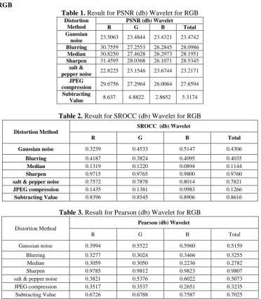
Figure 1. Comparison between different methods
1.5.HIS
Table 5. Result for PSNR (db) Wavelet for HIS
Table 6. Result for Pearson (db) Wavelet for HIS
Distortion Method
SROCC (db) Wavelet
H S I Total
Gaussian noise 0.0943 0.4239 0.3397 0.2860
Blurring 0.0868 0.3410 0.4142 0.2807
Median 0.0710 0.0797 0.1294 0.0934
Sharpen 0.4251 0.9660 0.9678 0.7863
salt & pepper
noise 0.9286 0.8388 0.7594 0.8423
JPEG
compression 0.0075 0.0849 0.1414 0.0729
Subtracting
Value 0.9361 0.8863 0.8384 0.7693
In HIS, also the best result is get for prewitt method but here the distortion method is Gaussian noise distortion method.
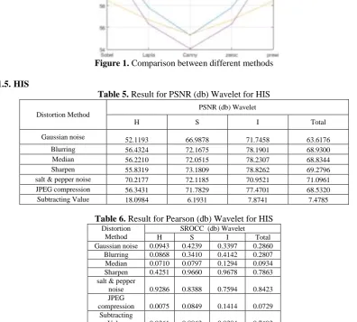
Figure 2. Comparison between different methods
Distortion Method
PSNR (db) Wavelet
H S I Total
Gaussian noise 52.1193 66.9878 71.7458 63.6176
Blurring 56.4324 72.1675 78.1901 68.9300
Median 56.2210 72.0515 78.2307 68.8344
Sharpen 55.8319 73.1809 78.8262 69.2796
salt & pepper noise 70.2177 72.1185 70.9521 71.0961
JPEG compression 56.3431 71.7829 77.4701 68.5320
V. Conclusion
Due to the Increase of the usage of digital image technology, computational speed etc., digital images have become important. These digital images go through various stages such as capturing, storing, transmitting, displaying etc. Thus, determining the image quality become a very important issue because distortions occur in these stages. Therefore, main target of modern multimedia systems design is to achieve a satisfying quality that the user can perceive. Image Quality Assessment (IQA) tries to quantify a visual quality or an amount of distortion in a given picture. Thus, IQA has become outstanding topic in research areas over the last years. Every year, number of new IQA algorithms is getting increase and extensions of existent algorithms are developed. But IQA is a difficult process which performs in image processing field and there is no highly efficient method yet. In this paper, an efficient quality metric which based on edge intensity of each pixel is clarified and applicator.
References
[1] H. Maitre, "A Review of Image Quality Assessment with application to Computational Photography," 2015.
[2] Chandler, "Seven Challenges in Image Quality Assessment: Past, Present, and Future Research," ISRN Signal
[3] Processing, 2012.
[4] C. B. Zhou Wang, LigangLu, "WHY IS IMAGE QUALITY ASSESSMENT SO DIFFICULT?," IEEE,
[5] 2002.
[6] J. A. Karen Egiazarian, Nikolay Ponomarenko, Vladimir Lukin, Federica Battisti, Marco Carli, "A New Full
[7] Reference Image Quality Metric Based on HVS."
[8] S. B. Sumit Mittal, "Objective Full Reference Image Quality Assessment Metrics," International Journal of
[9] Advanced Research in Computer Science, 2011.
[10] X. F. Xuande Zhang, Weiwei Wang, Wufeng Xue, "Edge Strength Similarity for Image Quality Assessment,"
[11] IEEE SIGNAL PROCESSING LETTERS, vol. 20, 2013.
[12] M. K. Jr., "Image Quality Assessment," WDS'12 Proceedings of Contributed Papers, 2012.
[13] C. B. Mohammed Hassan, "Evaluation of Image Quality Assessment Metrics Color Quantization Noise,"
[14] International Journal of Applied Information Systems (IJAIS), vol. 9, 2015.
[15] C. B. Zhou Wang, LigangLu, "Applications of Objective Image Quality Assessment Methods," IEEE
[16] SIGNAL PROCESSING MAGAZINE, 2011.
[17] Q. Huynh-Thu and M. Ghanbari, "Scope of validity of PSNR in image/video quality assessment," Electronics
[18] letters, vol. 44, pp. 800-801, 2008.
[19] Oriani, "qpsnr: A quick PSNR/SSIM analyzer for Linux," ht tp://qpsnr. youlink. org/).. Retrieved, vol. 6,
[20] 2011.
[21] S. Anitha and B. D. Nagabhushana, "Quality assessment of resultant images after processing," The International
[22] Institute for Science, Technology and Education (IISTE), vol. 3, pp. 105-112, 2012.
[23] S. T. Welstead, Fractal and wavelet image compression techniques vol. 40: Spie Press, 1999.
[24] Y. Fisher, "Fractal image compression," Fractals, vol. 2, pp. 347-361, 1994.
[25] N. Thomos, N. V. Boulgouris, and M. G. Strintzis, "Optimized transmission of JPEG2000 streams over wireless
[26] channels," IEEE Transactions on image processing, vol. 15, pp. 54-67, 2006.
[27] X. Li and J. Cai, "Robust transmission of JPEG2000 encoded images over packet loss channels," in Multimedia
[28] and Expo, 2007 IEEE International Conference on, 2007, pp. 947-950.
[29] D. Salomon, Data compression: the complete reference: Springer Science & Business Media, 2004.
[30] Lehman, N. O’Rourke, L. Hatcher, and E. Stepanski, "JMP for basic univariate and multivariate statistics,"
[31] SAS Institute Inc., Cary, NC, p. 481, 2005