ABSTRACT: The paper demonstrates the application of TOPSIS method using two selected examples. In the

(1)

ISSN (Online): 2320-9364, ISSN (Print): 2320-9356

www.ijres.org Volume 1 Issue 2

ǁ

June. 2013

ǁ

PP.05-12

Notes on TOPSIS Method

Zlatko Pavić

1

, Vedran Novoselac

2

1,2_{(Mechanical Engineering Faculty in Slavonski Brod, University of Osijek, Croatia)}

ABSTRACT: The paper demonstrates the application of TOPSIS method using two selected examples. In the

first example, it is shown that the best TOPSIS solution is neither closest to the positive ideal solution nor the farthest from the negative ideal solution. In many works on TOPSIS method stands as follows: "The basic principle is that the chosen alternative should have the shortest distance from the positive ideal solution and the longest distance from the negative ideal solution".

Keywords: decision matrix, negative ideal solution, positive ideal solution

I. INTRODUCTION

Multi-criteria decision making.

In a general sense, it is the aspiration of human being to make "calculated" decision in a position of multiple selection. In scientific terms, it is the intention to develop analytical and numerical methods that take into account multiple alternatives with multiple criteria.

TOPSIS (Technique for Order Preference by Similarity to Ideal Solution) is one of the numerical methods of the multi-criteria decision making. This is a broadly applicable method with a simple mathematical model. Furthermore, relying on computer support, it is very suitable practical method. The method is applied in the last three decades (on the history of TOPSIS see [4], [3]), and there are many papers on its applications (see [11], [8], [9]).

Description of the problem.

Given

m

options (alternatives)

A

_i, each of which depends on

n

parameters (criteria)

x

_j whose values are expressed with positive real numbers

x

_ij. The best option should be selected.

Mathematical model of the problem.

Initially, the parameter values

x

_ij should be balanced according to the procedure of normalization. Suppose that

a

_ij are the normalized parameter values. Then each option

A

_i is expressed as the point

1

(

,

)

n

i i in

A a

a



R

. Selecting the most optimal value

a

_j



{

a

₁_j

,

a

_mj

}

for every parameter

x

_j, we determine the positive ideal solution

A



= (

a

₁

,

a

_n

)

. The opposite is the negative ideal solution

1

= (

,

n

)

A



a



a

 . The positive and negative ideal solution are also denoted by

A

 and

A

. The decision on the order of options is made respecting the order of numbers

( ,

)

1 =

=

.

( ,

)

( ,

)

( ,

) / ( ,

) 1

i i

i i i i

d A A

D

d A A

 



_

  

_

(1)

The option

1

i

A

is the best solution if ₁ ₂

1

max{

D D



,



,

D

_m

} =

D

_i



, and the option

2

i

A

is the worst solution

if ₁ ₂

2

min{

D D



,



,

D

_m

} =

D

_i



. The other options are between these two extremes. The maximum distance

=1, ,

= max

i m i

D



D

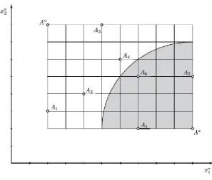
 is usually called TOPSIS metric.

Geometrical image of the problem.

(2)

is the alternative

A

₇.

Figure 1. Geometrical representation of TOPSIS method

TOPSIS is a compensatory method. These kinds of methods allow the compromise between different criteria, where a bad result in one criterion can be compensated by a good result in another criterion. An assumption of TOPSIS method is that each criterion has either a monotonically increasing or decreasing preference. Due to the possibility of criteria modelling, compensatory methods, certainly including TOPSIS, are widely used in various sectors of multi-criteria decision making (see [10], [2], [1]).

II. COMPUTATIONAL PROCEDURE FOR TOPSIS METHOD

Problem.

We examine

m

alternatives

A

₁

,

A

_m. Each alternative

A

_i respects

n

criteria

x

₁

,

x

_n which are expressed with positive numbers

x

_ij. The criteria

x

₁

,

x

_k are benefit (monotonically increasing preference), and criteria

x

k₁

,

x

n are non-benefit (monotonically decreasing preference). Weights

w

j of the criteria

x

j are given so that

=1

= 1

n j j

w



. It is necessary to select the most optimal alternative. Initial Table and Decision Matrix.

For better visibility, the given alternatives, criteria and its weights are placed in the table (see Table 1).

(3)

The given numbers

x

_ij and their matrix

11 12 1

21 22 2

1 2

=

n

m m mn

x

































X

(2)

must be balanced, since the numbers

x

_ij present values of different criteria with different measuring units. One must also take into account the given weights

w

_j of the criteria

x

_j. First, the measuring numbers

x

_ij of the criteria

x

_j are replaced with the normalized or relative numbers

2 =1

=

ij

ij _m

ij i

x

r

x



(3)

belonging to the open interval

 

0,1

. Then, according to the share

w x

_j _j of the criteria

x

_j, the normalized numbers

r

_ij are replaced with the weighted normalized numbers

2 =1

=

ij

ij j ij j _m

ij i

x

a

w r

w

x



(4)

belonging to

 

0,1

. The further data processing uses the weighted normalized decision matrix

11 12 1

21 22 2

1 2

=

.

n

m m mn

a

































A

(5)

If all weights

w

_j are mutually equal, in which case

w

j

= 1 /

n

, the numbers

r

ij can be applied in the matrix

A

as the numbers

a

_ij.

Working Table.

The weighted normalized decision matrix

A

and all the data that will be calculated, we try to write in one table.

(4)

The coordinates

a

_j of the positive ideal solution

A

= (

a a

₁ ₂

a

n

)

   

are chosen using the formula

for

= 1,

,

max

=

min

for

=

1,

, .

ij i

j ij

i

a

j

k

a



a

j

k

n





_







(6)

If some alternative

0

i

A

is equal to

A

, then it is obvious that the alternative

0

i

A

is the best solution. If it is not, then we continue the procedure.

The coordinates

a

_j of the negative ideal solution

A

= (

a a

₁ ₂

a

n

)

   

are chosen applying the formula

for

= 1,

,

min

=

max

for

=

1,

, .

ij i

j ij

i

a

j

k

a



a

j

k

n





_







(7)

The numbers

d

_i of the column

d

= (

d d

₁ ₂

d

m

)

    

are the distances from the points

A

_i to the point

A

, which is calculated by the formula





2

=1

= ( ,

) =

.

n

i i ij j

j

d



d A A





a



a

 (8)

The numbers

d

_i of the column

d

= (

d d

₁ ₂

d

m

)

    

are the distances from the points

A

_i to the point

A

, which is calculated by the formula





2

=1

= ( ,

) =

.

n

i i ij j

j

d



d A A





a



a

 (9)

The numbers

D

_i of the column

D

= (

D D

₁ ₂

D

m

)

    

are the relative distances of the points

A

_i respecting the points

A

 and

A

, which is expressed by the formula

( ,

)

=

.

( ,

)

( ,

)

i i i

i i i i

d

d A A

D

d

d A A

 



_

 

_

 (10)

If ₁ ₂

1

max{

D D



,



,

D

_m

} =

D

_i



, then we accept the alternative

1

i

A

as the best solution. If

1 2 ₂

min{

D D



,



,

D

_m

} =

D

_i



, then we accept the alternative

2

i

(5)

III. TWO EXAMPLES OF USING TOPSIS METHOD

Example 1. Four alternatives with three criteria are given in Table 3. The criteria

x

₁ and

x

₂ are benefit, and the criterion

x

₃ is non-benefit. The weights of the criteria are equal. Decide which alternative is the best.

Table 3. Initial table for Example 1

Since the weights are equal, we can use the normalized decision matrix

A

with the elements

4 2 =1

=

ij

ij i

x

a

x



(11)

for

i

= 1, 2,3, 4

and

j

= 1, 2,3

. In this case, the matrix

A

reads as follows:

0,535

0, 441 0, 407

0, 688

0, 441 0, 488

=

0,382

0,515

0, 732

.

0,306

0,588

0, 244

































A

(12)

Relying on the matrix

A

, we have to determine two rows (

A

,

A

) and three columns (

d

,

d

,

D

) in the working table.

Table 4. Working table for Example 1

According to the formula in (6), the positive ideal solution

A



= (

a a a

₁  ₂ ₃

)

contains the greatest numbers of the first and second column of

A

, and the smallest number of the third column of

A

.

According to the formula in (7), the negative ideal solution

A



= (

a a a

₁ ₂ ₃

)

contains the smallest numbers of the first and second column of

A

, and the greatest number of the third column of

A

.

(6)

by the formula in (8) with

n

= 3

, so





3 ₂

=1

= ( ,

) =

.

i i ij j

j

d



d A A





a



a

 (13)

The distances

d



= (

d d d d

₁ ₂ ₃ ₄ 

)

, from the alternatives

A

_i to the negative ideal solution

A

, are calculated by the formula in (9) with

n

= 3

, so





3 ₂

=1

= ( ,

) =

.

i i ij j

j

d



d A A





a



a

 (14)

The relative distances

D



= (

D D D D

₁ ₂ ₃ ₄ 

)

of the alternatives

A

_i respecting the positive ideal solution

A

 and negative ideal solution

A

 are calculated using the formula in (10), so

=

i

.

i

i i

d

D

d

 



_

 (15)

Applying the last tree columns of the Table 4 we have the following three preferred orders of alternatives:

A A A A

2 1 4 3 by the column of

D



from the largest to smallest number

A A A A

d



A A A A

d



from the smallest to largest number TOPSIS method prefers the first order respecting the column of

D

.

In the following example we have the most desirable combination:

d

,

d

 and

D

 point to one and the same best solution.

Example 2. 1Six alternatives with five criteria and their weights are given in Table 5. The criteria

x x x

₁

,

₂

,

₃ are benefit, and the criteria

x x

₄

,

₅ are non-benefit. Select the best alternative.

Table 5. Initial table for Example 2

Weighted normalized decision matrix

A

with the elements

6 2 =1

=

ij

ij j

ij i

x

a

w

x



(16)

(7)

0,118

0, 049

0, 057

0,118

0, 033

0,158

0, 035

0, 043

0,103

0, 088

0, 097

0, 028

0,113

0, 044

0, 077

=

.

0, 079

0, 063

0, 099

0, 088

0, 055

0,178

0, 028

0, 071

0,103

0, 066

0, 059

0, 028

0, 085

0,133

0, 022





































A

(17)

The positive ideal solution

A



= (

a a a a a

₁    ₂ ₃ ₄ ₅

)

contains the greatest numbers of the first, second and third column of

A

, and the smallest numbers of the fourth and fifth column of

A

.

The negative ideal solution

A



= (

a a a a a

₁ ₂ ₃ ₄ ₅

)

contains the smallest numbers of the first, second and third column of

A

, and the greatest numbers of the fourth and fifth column of

A

.

The distances

d



= (

d d d d d d

₁ ₂ ₃ ₄ ₅ ₆ 

)

A

_i to the positive ideal solution

A

, are calculated applying the distance formulas in (8) with

n

= 5

.

The distances

d



= (

d d d d d d

₁ ₂ ₃ ₄ ₅ ₆ 

)

A

_i to the negative ideal solution

A

, are calculated applying the distance formulas in (9) with

n

= 5

.

The relative distances

D



= (

D D D D D D

₁ ₂ ₃ ₄ ₅ ₆ 

)

of the alternatives

A

_i respecting the positive ideal solution

A

 and negative ideal solution

A

 are determined using the quotient formulas in (10).

Table 6. Working table for Example 2

Applying the last tree columns of the Table 6 we have the following three preferred orders of alternatives:

A A A A A A

5 3 2 4 1 6 by the column of

D



A A A A A A

d



A A A A A A

d



from the smallest to largest number

(8)

IV. CONCLUSION

In the method presenting it is important to find examples that adequately show its meaning and application. After that, the generalizations of the method can be implemented to extend its applications. In the case of TOPSIS method the first generalization refers to the processing of insufficiently precise data, namely, fuzzy data (see [6], [5], [1]).

The second generalization applies to the norm and metric. Let

p



1

be a real number. Using the

p

-norm in the normalization procedure, we get

1

=1

=

.

|| (

,

) ||

|

ij ij

ij _m

j mj p _p p

ij i

x

r

x



(18)

Then, using the

p

-metric in the distance calculation, we have

=1

=

( ,

) =

|

| .

n

p p

i p i ij j

j

d



d

A A





a



a

 (19)

The max-norm and max-metric can also be applied in the computational procedure of TOPSIS method .

REFERENCES

[1] A. Balin, P. Alcan, and H. Basligil, Co performance comparison on CCHP systems using different fuzzy multi criteria decision making models for energy sources, Fuelling the Future, pp. 591-595, 2012.

[2] I. B. Huang, J. Keisler, and I. Linkov, Multi-criteria decision analysis in environmental science: ten years of applications and trends, Science of the Total Environment 409, pp. 3578-3594, 2011.

[3] C. L. Hwang, Y. J. Lai, and T. Y. Liu, A new approach for multiple objective decision making, Computers and Operational Research 20, pp. 889-899, 1983.

[4] C. L. Hwang, and K. Yoon, Multiple Attribute Decision Making: Methods and Applications, Berlin Heidelberg New York, Springer-Verlag, 1981.

[5] G. R. Jahanshahloo, F. Hosseinzadeh Lotfi, and M. Izadikhah, Extension of the TOPSIS method for decision-making problems with fuzzy data, Applied Mathematics and Computation, pp. 1544-1551, 2006. [6] Y. J. Lai, T. Y. Liu, and C. L. Hwang, Fuzzy Mathematical Programming: Methods and Applications, Berlin

Heidelberg New York, Springer-Verlag, 1992.

[7] Y. J. Lai, T. Y. Liu, andC. L. Hwang, TOPSIS for MODM, European Journal of Operational Research 76, pp. 486-500, 1994.

[8] G. H. Tzeng, and J. J. Huang, Multiple Attribute Decision Making: Methods and Applications, New York, CRC Press, 2011.

[9] J. Xu, and Z. Tao, Rough Multiple Objective Decision Making, New York, CRC Press, 2012.

[10]K. A. Yoon, A reconciliation among discrete compromise situations, Journal of Operational Research Society 38, pp. 277-286, 1987.

[11]K. P. Yoon, and C. Hwang, Multiple Attribute Decision Making: An Introduction, California, SAGE Publications, 1995.