A Novel Strategy for Mining Frequent Closed
Itemsets in Data Streams
Keming Tang
College of Computer Science and Technology, Nanjing University of Aeronautics and Astronautics, Nanjing, China Department of Software Engineering, Yancheng Teachers University, Yancheng, China
Caiyan Dai
College of Computer Science and Technology, Nanjing University of Aeronautics and Astronautics, Nanjing, China [email protected]
Ling Chen*
Department of Computer Science, Yangzhou University, Yangzhou, China [email protected]
Abstract— Mining frequent itemsets from data stream is an important task in stream data mining. This paper presents an algorithm Stream_FCI for mining the frequent closed itemsets from data streams in the model of sliding window. The algorithm detects the frequent closed itemsets in each sliding window using a DFP-tree with a head table. In processing each new transaction, the algorithm changes the head table and modifies the DFP-tree according to the changed items in the head table. The algorithm also adopts a table to store the frequent closed itemsets so as to avoid the time-consuming operations of searching in the whole DFP-tree for adding or deleting transactions. Our experimental results show that our algorithm is more efficient and has lower time and memory complexity than the similar algorithms Moment and FPCFI-DS.
Index Terms— Stream data, mining closed frequent data itemsets, sliding window
I. INTRODUCTION
In recent years, researchers have paid more attention to mining data streams. Mining frequent itemsets from data streams is an important problem with ample applications in data streams analysis. Examples include stock tickers, bandwidth statistics for billing purposes, network traffic measurements, web-server click streams, data feeds from sensor networks, transaction analysis in stocks and telecom call records, etc. Unlike traditional data sets, data streams flow in and out of a computer system continuously and with varying update rates. They are temporary ordered, fast changing, massive and potentially infinite. For the stream data applications, the volume of data is usually too huge to be stored or to be scanned for more than once. Furthermore, since the data items can
only be sequentially accessed in data streams, random data access is not practicable.
In 1999, Pasquierti[1] first proposed the concept of closed frequent data itemsets to reduce the storage space and processing time. Since then mining closed frequent data itemsets has been the subject of numerous studies. Many of the algorithms proposed in these studies are Aperiori-based[2]. They depend on a generate-and-test paradigm. They find frequent itemsets from the transaction database by first generating candidates and then checking their supports against the transaction data base.
To improve efficiency of the mining process, Han et al[3] proposed an algorithm FP-growth (frequent-pattern growth) which is a tree-based algorithm for finding frequent itemsets. FP-growth algorithm is based on the following partition strategy. Firstly it compresses the database into a frequent pattern tree. Then the compressed database is divided into a group of conditional database, each of which is associated with a frequent itemset or a pattern portion and then the algorithm mines every conditional database. To construct the FP-tree, the database must be scanned twice. Like the Apriori approach, the first scan generates the frequent 1-itemsets and their supports. The results are sorted in the descending order of their supports and stored in a list L. In the second scan, transactions are processed by the order in the list L and a branch in FP-tree is created for each transaction. To traverse the tree easily, a head table is constructed where each item has a pointer indicating its node in the FP-tree.
conditional pattern tree. The algorithm needs not to generate all the candidate frequent itemsets. It uses the most infrequent item as the suffix to reduce the search space and the overhead significantly.
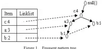
Example 1: Let I ={a,b,c,d}, D={ac,bc,abc,acd}, min_sup=2, then L={{c:4},{a:3},{b:2}}, the generated FP-tree is shown in Fig.1.
When mining the closed frequent itemsets in a static database, FP-growth algorithm needs to scan the database more than once. It is not practicable in data stream mining which allows only one time scan.
For mining the frequent itemsets in data stream, MOMENT by Chi[4] is a typical algorithm which can decrease the size of the data structure. In solving many application problems, it is desirable to discount the effect of the old data. One way to handle such problem is using sliding window models. There are two typical models of sliding window[5]: milestone window model and attenuation window model. Lossy Counting[6] is a typical mining algorithm for data streams based on the milestone window. Using the attenuation window, Chang presented the algorithm Decest[7]. Gannell[8] proposed FP-stream by adopting the traditional FP-tree to process the data streams. FP-stream detects the frequent itemsets in the different period by using the different time granularity. Key differences between tree and FP-stream structure include the following. First, each path in an FP-tree represents a transaction, while each path in an FP-stream represents a potential frequent itemset. Second, each node in an FP-tree contains one support value, whereas each node in an FP-strean contains a nature or logarithmic tilted-time window table containing multiple support values, one for a batch of transactions. Teng proposed FTP-DS algorithm[9] which uses the statistical regression technique in the sliding window. Fujiang Ao et al[10] presented an algorithm named FPCFI-DS for mining closed frequent itemsets in data streams. FPCFI-DS uses a single-pass lexicographical-order FP-Tree-based algorithm with mixed item lexicographical-ordering policy to mine the closed frequent itemsets in the first window, and updates the tree for each sliding window.
In this paper, we present an algorithm Stream_FCI for mining the frequent closed itemsets from data streams in the model of sliding window. The algorithm detects the frequent closed itemsets in each sliding window using a DFP-tree (Dynamical FP-tree) with a head table. In processing each new transaction the algorithm changes the head table and modifies the DFP-tree according to the changed items in the head table. The algorithm also adopts a table FCIT (frequent closed itemset table) to store the frequent closed itemsets so as to avoid the time-consuming operations of searching in the whole DFP tree for adding or deleting transactions. The frequent closed itemsets are first arranged in FCIT in the descending order of their supports. For the frequent closed itemsets with identical support in FCIT, they are organized in a lexicographical order. When adding or deleting transactions, DFP-tree and FCIT should be updated
accordingly. In DFP-tree, the nodes in every path are arranged in the descending order of their supports so as to reduce the searching space in maintaining and mining the DFP-tree. Our experimental results show that the algorithm is more efficient and has lower time and memory complexity than the algorithms Moment and FPCFI-DS.
The rest of this paper is organized as follows. The next section describes the background of frequent closed itemset mining. In section 3, our algorithm Stream_FCI is introduced. Section 4 shows the experimental results in testing Stream_FCI. Finally, conclusions are given in Section 5.
II. BACKGROUND
A. Frequent Closed Itemsets
Let I ={i1,i2,",im} be a set of distinct data items,
and a subset X⊆I is called an itemset. Each transaction
t is a set of items in I . A data stream,
),...}
,
(
),...,
,
{(
tid
1t
1tid
nt
nDS
=
, is an infinitesequence of transaction, where tidk is the identifier of a transaction and tk ⊆I(k=1,2,",n) is an itemset. For all
transactions in a given window W of data stream, the
support
sup(
X
)
of an itemset X is defined as thenumber of transactions with X as a subset.
Figure 1. Frequent pattern tree.
Given a threshold of support min_sup in the range of [0,w], where w is the size of the sliding window, the itemset X is frequent if sup(X)≥min_sup.
In general, the more transactions a sliding window has, a larger amount of frequent itemsets could be produced. In this case, there are many redundancies among those frequent itemsets. For example, in the frequent itemsets
} , ,
{acd ad a , the only useful information is set acd
according to Apriori[2] property, because acd includes ad and a . Closed itemsets are a solution to this problem. A frequent itemset X is a closed one if it has no superset Y ⊃X such thatsup(X)=sup(Y). Closed
possible to derive the identity and the support of every frequent itemset in the collection from them. Since when mining closed itemsets, we implicitly discard redundancies, extracting association rules directly from them has been proven to be more meaningful for analysis.
Example 2: Let I ={a,b,c,d}, D={ac,bc,abc,acd}, min_sup=2. The frequent itemsets are (a:3), (b:2), (c:4), (ac:3) and (bc:2). Since (a:3) has the same support with its superset (ac:3), (b:2) has the same support with its superset (bc:2), they are not frequent closed itemsets. Therefore, the frequent closed itemsets are (c:4), (ac:3) and (bc:2).
B. Sliding Window
In some real world applications such as meteorological study and financial operations, recent data in the stream have more importance than the old ones. One way to handle such problem is using a fading factor to act on the count of data items in data stream. It takes into account all the old data items in the history, and assigns less weights on the past data. In some applications, the users are interested in the current data within a fixed time period. Therefore, the sliding window[5] is another practical approach to emphasis the recent data in the stream. It is suitable for the applications such like stocks or sensor networks, where only recent events may be important. The sliding window model only observes within a limited time window and entirely ignores the ones outside. This method reduces memory requirements because only a small portion of data is stored.
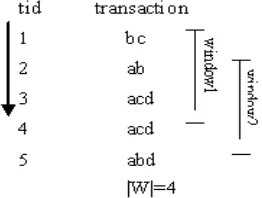
The basic idea of mining frequent closed itemset in the sliding window model is that it makes decisions from the recent transactions in a fixed time period instead of all the transactions happened so far. Formally, a new data element arriving at the time t will expire at time , where is the length of the window. At every time step, when a new transaction comes to the window, the oldest one in the window should be deleted. Since the transactions in the window are updated over time, the frequent itemsets should be renewed accordingly. Fig.2 shows an example of sliding window. Since the model only stores the data items within a small data window of fixed size, it needs less memory space and is easy to be implemented.
Figure 2. An example of sliding window.
III. THESTREAM_FCIALGORITHM
In this section, we illustrate the frame work of the algorithm Stream_FCI for mining the frequent closed itemsets in data streams based on the model of sliding window. First the data structure used in the algorithm is introduced.
A. Data Structure
(1) DFP-tree (Dynamical frequent-pattern tree)
To construct the conventional FP-tree, the database must be scanned twice. However, it is not suitable for processing the stream data. A data structure called DFP (Dynamical frequent-pattern tree) is proposed to store the transactions in the current sliding window.
The root of the tree is labeled with null. A branch starting from the root is created for each transaction. The itemstes sharing the common prefix will have identical ancestors in their paths. Each node on the tree represents an item. The structure of each node x in the tree is as follows:
node_item node_sup node_link
Here, node_item(x) is the the name of the item in the node x; node_sup(x) is the count of the item in node x ; node_link(x) is the pointer of the item linking with the other items which having the same node_name.
A transaction is represented in DFP-tree by a path starting from the root. To make the algorithm be suitable for data streams and reduce the memory cost, items in each transaction are arranged in its path in the order of descending support count. In general the count of each node along the common prefix is greater than the summation of the counts of its child nodes.
(2) Head Table
To facilitate the tree traversal, a head table is built so that each item points to its occurrences in the tree via a chain of node links. The head table stores all the frequent items which may be consisted in the frequent closed itemsets in the DFP-tree.
Every record in the head table represents an item, and its structure is as follows:
sup item_name link
Here, sup is the count of the item, item_name is the name of the item, and link is the pointer which is linked with the chain of nodes of item_name in DFP-tree.
To make the algorithm be suitable for data streams and efficient in terms of memory and time cost, the entries in the head table are arranged in a descending order of their supports. All the possible items are considered as alphabets which form an alphabet table ∑. The items with the same count are arranged according to their alphabetical order.
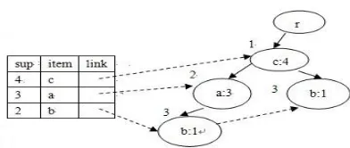
Figure 3. A dynamical frequent pattern tree.
(3) Frequent Closed Itemsets Table (FCIT)
In in order to record the frequent closed itemsets, a table called FCIT (Frequent Closed Itemsets Table) is used, where each entry records the count of a frequent closed itemset. The structure of each entry in the table is as follows:
sup set
Here, sup is the count of the frequent closed itemset; set is the frequent closed itemset.
In FCIT, the entries are arranged in the order as follows. Firstly, the items in each itemsets are arraged according their alphabet order in ∑, which is called the the normal expression of the itemset. The entries in the FCIT are arranged by the descending order of their counts. The itemsets with the same count are arranged in the lexical order of their the normal expression defined on ∑.
In fact, each entry (sup, set) can be treated integractively as a vector, and all those vectors are arranged in FCIT according to their lexical order. We can perform radix sorting and binary search on FCIT so as to make quick querys and modifications on the table.
Example 4: The frequent closed itemsets of the transactions in Example 3 are {c:4}, {ac:3}, {bc:2}. Their FCIT TABLE I is as follows:
TABLE I. FCIT
sup set
4 c
3 ac
2 bc
B. Framework of algorithm Stream_FCI
The algorithm Stream_FCI receives a transaction from the data stream at each time step, and forms a new sliding window by adding this new transaction into the window and emitting the oldest one. To identify the frequent closed itemstes in this new sliding window, Stream_FCI should modify the DFP-tree, head table and FCIT accordingly. Since two adjacent windows are overlapped except the added and deleted transactions, the frequent
closed itemsets of the two windows do not change abruptly. Stream_FCI needs only to process the part of DFP-tree, head table and FCIT involving these two transactions. Therefore, procedures are proposed to modify DFP-tree, head table and FCIT when adding and deleting a transaction.
At the beginning of the stream, DFP-tree, head table and FCIT are firstly constructed for the first window using a procedure BuildFirstTree.
The framework of algorithm Stream_FCI(D) is as follows:
Algorithm: Stream_FCI(D)
Input: D: the data stream;
Output: L: the frequent closed itemset table; Begin
1 BuildFirstTree(T);
2 while not the end of the stream do
3 Receive a new transaction t from the stream; 4 AddTransDFP(T,t);
5 Adjust(T);
6 AddTransFCIT(L,t); 7 DeleteTransDFP(T,s); 8 Adjust(T);
9 DeleteTransFCIT(L,s)
/* s is the oldest transaction in the window*/ 10 endwhile
End.
C. Constructing the first DFP-tree and FCIT
The DFP-tree and FCIT for the first window are constructed by a procedure BuildFirstTree(). When a new transaction in the stream enters the first window, the head table is modified by increasing the supports of the items in the new transaction. Then the new transaction will be inserted into the DFP-tree according to the pointers of its items listed in the head table. A procedure AddTransDFP(T,t) is presented to add a new transaction t into the DFP-tree rooted at T. Also, the FCIT table is modified accordingly by adding the new frequent closed itemsets detected in the DFP-tree. A procedure AddTransFCIT(L,t) is presented to modify the FCIT table L when adding a new transaction t.
The algorithm BuildFirstTree() is described as follows:
Procedure: BuildFirstTree()
Input: length: length of the window; Output: T: the root of DFP-tree,
L: the frequent closed itemsets table
Begin
1 T=Φ; size=0; 2 repeat
3 receive a new transaction t from the stream; 4 update the head table;
Details of procedures AddTransDFP(T,t) and AddTransFCIT(L,t) will be diescribed in the next section.
D. Adjusting the DFP-tree
After adding or deleting a new transaction, since the supports of the items are changed, the DFP-tree should be adjusted accordingly so that the nodes in each path of the tree are arranged in the descending order of their supports. A procedure Adjust(T) is proposed to rearrange the nodes in DFP-tree.
Suppose node y in DFP-tree is a child of node x, and node_item(x)=a, node_item(y)=b. If in the head table sup(a)<sup(b), then x and y can be called an inversed pair. Suppose node x and y is an inversed pair, the position of x and y should be exchanged to make sure they are in the descending order of their supports. In DFP-tree, the subtree rooted at node x is denoted as subtree(x), and let subtree-(x)=subtree(x)-{x}. When
exchanging the position of an inversed pair of nodes, if node y is the only child of x, their position can be exchanged directly. But if x has children other than y, subtree-(y) should be inserted into w, which is the father
of node x, and the support of x should be modified accordingly.
The procedure Adjust(T) is described as follows:
Procedure: Adjust(T)
Input: T: root of the DFP-tree
Output: the adjusted DFP-tree rooted at T. Begin
1 while there exists inversed pair in T do
/* Suppose the inversed pair is (x,y), y is the child node of x , w is the parent of x */ 2 Delete subtree(y) from the children set of x; 3 node_sup(x)=node_sup(x)-node_sup(y);
4 Add a path “u→ v→subtree-(y)” as a child of w;
5 node_item(u)=node_item(y); 6 node_sup(u)=node_sup(y); 7 node_item(v)=node_item(x); 8 node_sup(v)=node_sup(y); 9 if w has another child p such that
node_item(p)=node_item(u) then
10 emerge subtree(p) and subtree(u); 11 endif
12 endwhile End.
Let the length of the window be 4, Fig.4 illustrates the process of constructing the first DFP-tree of the database in Fig.2. In Fig.4, (a), (b) , (c) and (d) show the changing of DPF-tree when the first four transactions are inserted, while (e) is the FCIT TABLE II for the first sliding window.
(a) Inserting transaction.bc
(b) Inserting transaction.ab
(c) Inserting transaction.acd
(d) Inserting transaction.acd
TABLE II. FCIT
sup set
3 a
3 c
2 acd
2 b
(e) The FCIT TABLE II
Figure 4. Building the first DFP-tree and FCIT TABLE II.
When the fourth transaction coming into the sliding window, supports of a, b and c can be found, which are identical in the previous window, have been changed. The supports of a and c in the new window are greater than that of b. Therefore, locations of their nodes in the DFP-tree should be rearranged by the procedure Adjust(T). The process of rearranging the nodes in DFP-tree is shown in Fig.5.
(b) Merging the same nodes.
(c) Exchange b and.c
Figure 5. Rearrange the order of the nodes in DFP-tree.
E. Adding a Transaction
When a new transaction enteres the sliding window, it should be added into DFP-tree and FCIT should be modified accordingly. A procedure AddTransDFP(T,t) is presented to add a new transaction into the DFP-tree. Also a procedure AddTransFCIT(T,t) is presented to modify the FCIT table when adding a new transaction.
(1) AddTransDFP(T,t)
The procedure AddTransDFP(T,t) is to add a new transaction t into the DFP-tree rooted at T. When a transaction is to be added into the DFP-tree, its items are processed in order according to descending support count. Suppose the first item of the inserted transaction t is b, the algorithm first finds a child of T representing item b, and then recursively constructs the path according to the rest part of t. If T has no such a child representing item b, a new child of T representing item b is created.
The procedure AddTransDFP(T,t) is shown as follows:
Procedure: AddTransDFP(T,t)
Input: T: Root of the DFP-tree
t: The transaction to be added
Output: the updated DFP-tree rooted at T Begin
/* Suppose t=(b|B), b is the first item in t, B is the suffix of t after b */ 1 if T has a child x such that node_item(x) =b then
2 node_sup(x)=node_sup(x) +1; 3 else create a new node x as a child of T;
4 node_sup(x)=1; 5 node_item(x)=b;
6 make node_link(x) to the end of link b 7 end if
8 if B is not empty then
9 AddTransDFP(x,B); 10 end if
End.
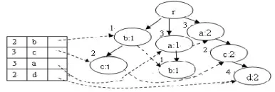
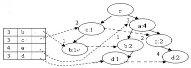
Fig.6 shows the new DFP-tree after inserting new transaction into the current window of Fig.5.
Figure 6. The DFP-tree after inserting.abd
When new transaction abd is received, the algorithm detects if there exists a child of root T representing item a. Since node (a:3) has already exists in DFP-tree, the algorithm modifies (a:3) into (a:4) and detects if it has a child representing item b. Since node (b:1) has already exists, the algorithm modifies (b:1) into (b:2) and detects if it has a child representing item d. Since (b:2) has no child, the algorithm simply adds a child node (d:1). The pointer of item d in head table is modified accordingly.
(2) AddTransFCIT(L,t)
When a new transaction enters the data stream, FCIT should be modified accordingly by adding the new frequent itemsets detected in the DFP-tree. A procedure AddTransFCIT(L,t) is presented to modify the FCIT table when adding a new transaction t.
When inserting a new transaction t, we first detect: 1) If there already exists the same itemset t in FCIT, its support should be increased by 1.
2) If the FCIT table has already included some sup-sets of the new transaction t, the new transaction t is a frequent closed itemset and should be inserted into FCIT. Its support is set equal to the support of the largest support of its supsets plus 1.
3) If there exists a subset r of the new transaction t in FCIT, support of r should be increased by 1.
The procedure of AddTransFCIT(L,t) is as follows:
Procedure: AddTransFCIT(L,t)
Input: L: the FCIT table;
t: The new transaction added;
Output: the updated frequent closed itemsets table L; Begin
1 if t is in L then sup(t)=sup(t)+1;
2 else
3 if there exists s which has the maximal
4 support in the supersets of t in FCIT then
5 add t into L; 6 sup(t)=sup(s)+1 7 else
8 Search t in the DFP-tree;
9 if t is a newly generated frequent closed
10 itemset then add t into L; 11 end if
12 end if
13 end if
14 for all subset r of t do
15 If there exists r in L then
17 else
18 Search r in the DFP-tree;
19 if r is a newly generated frequent closed
20 itemset then add r into L;
21 end if
22 end if
23 end for End.
F. Deleting a Transaction
Once a new transaction is added into the window, the oldest one in the window must be discarded, and the DFP-tree and FCIT table should be modified accordingly. A procedure DeleteTransDFP is presented to delete an old transaction from the DFP-tree. Also a procedure DeleteTransFCIT is presented to modify the FCIT table when deleting an old transaction.
(1) Delete TransDFP(L,t)
The procedure DeleteTransDFP(T,t) is to delete a transaction t from the DFP-tree rooted at T. Since each transaction in the DFP-tree is represented by a path starting from the root, to delete a transaction from the DFP-tree, the counts of the nodes on the path can be simply decreased. The procedure of DeleteTransDFP(T,t) is described as follows:
Procedure: DeleteTransDFP(T,t)
Input: T: Root of the DFP-tree;
t: The transaction to be deleted;
Output: the updated DFP-tree rooted at T; Begin
/* suppose t=[b|B]*/
1 Find node X in T’s children such that item(X)=b; 2 if such X exists then
3 node_sup(X)=node_sup(X)-1; 4 DeleteTransDFP(X,B); 5 end if
End.
Adding or deleting a transaction in the DFP-tree may cause disorder on the supports of the nodes in the paths. Therefore it is necessary to call procedure Adjust(T) to rearrange the nodes in the DFP-tree.
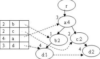
Fig.7 and Fig.8 illustrate the changes of DFP-tree after deleting transaction bc from the tree in Fig.6.
Figure 7. Deleting transaction bc from DFP-tree.
Figure 8. The change of DFP-tree after deleting.bc
(2) DeleteTransFCIT(L,t)
The procedure DeleteTransFCIT(L,t) is to delete a transaction t from the FCIT table L. Since no new frequent closed itemset could appear when deleting an old transaction, the number of the enties in FCIT will not increase. When deleting a transaction t, we should detect whether there exist t or the subsets of t in FCIT table. The set which consists of t and its subsets in FCIT are defined as F(t). If F(t) is not empty, the supports of all itemsets in F(t) should be decreased by 1, and may be removed from FCIT if such a itemset becomes infrequent or not closed. The procedure DeleteTransFCIT(L,t) is described as follows:
Procedure: DeleteTransFCIT(L,t)
Input: L: the FCIT table;
t: the transaction to be deleted;
Output: modified FCIT table L
Begin
1 Detect if there exist t and its subsets in L; /* define the set which consists of t
and its subsets in L as F(t) */ 2 if F(t) is not empty then
3 for each itemset r in F(t) do
4 sup(r)=sup(r)-1;
5 if sup(r)<minsup then delete r from L
6 else
7 if there exsits a superset s of r in L
8 such that sup(s)=sup(r) then 9 delete r from L;
10 end if
11 end if
12 end for
13 end if End.
The FCIT TABLE III of the second sliding window of database in Fig.1 is as follows:
TABLE III. FCIT
sup set
4 a
3 ad
2 ab
IV. EXPERIMENTALRESULTS
The quality and efficiency of our Algorithm Stream_FCI is evaluated through extensive experiments on the real data set and compare with algorithms Moment[4] and FPCFI-DS[10]. We focus on the algorithms’ memory costs, computation times for building the first window and the average time of the sliding window moving.
All experiments were carried out on a 2.8GHz CPU and 1G RAM PC running Windows version XP; the program developed in Visual studio C++6.0.
A. Test Data Sets
The testing datasets Mushroom[11] and T10I4D100K[11] are used. Mushroom is a dense dataset which contains 8124 pieces of records. T10I4D100K adopts three common parameters: T (the longest length of the transaction); I (the average length of the transaction); D (the number of the items in the datasets). The the longest length of the transactions in T10I4D100K is 10, and the average length of the transactions is 4, the number of the items in the datasets is 100K. Similar to [12], system tool is used to observe the change of the memory usage. The average time for processing the sliding window is obtained by 100 trials. The sizes of the sliding window are 5K and 60K for mining on dense and sparse dataset respectively.
B. Experimental Results and Analysis
The memory costs by Moment, FPCFI-DS and Stream_FCI are first compared. Fig.9 shows the memory requirements of the three algorithms. From the figure we can see that for processing both dense and sparse dataset, Moment requires the most memory space and Stream_FCI requires the least. The main reason is that Stream_FCI only searches in the DFP-tree to establish FCIT without generating all candidate itemsets or using an extra data array.
We also test the three algorithms to compare their times for building the first window. Fig.10 shows the test results, from which it can be seen that when minsup changes from 1 to 0.1, Stream_FCI is obviously faster than Moment, but a little slower than FPCFI-DS. The reason is that when building the first window, Stream_FCI needs to adjust the nodes in the DFP-tree so that the nodes in each path are arranged in the descending order of their supports. But after generating the first DFP-tree and the FCIT, Stream_FCI is faster than the other two algorithms.
(a) Mushroom.
(b) T10I4D100K.
Figure 9. Memory usage.
(a) Mushroom.
(b) T10I4D100K.
Figure 10. The time of building the first window.
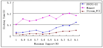
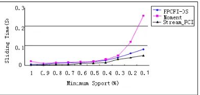
The comparison of the average time to processing each sliding window by the three algorithms is shown in Fig.11. The processing of one window consists of adding a new transaction entering the current window and deleting an old one from it. From Fig.11 it can be found that Stream_FCI is faster than other two algorithms especially when the value minsup is decreasing.
(b) T10I4D100K.
Figure 11. The average time of window sliding.
V. CONCLUSION
To mining the closed frequent itemsets in data streams, this paper presents an algorithm Stream_FCI on the model of sliding window. The algorithm detects the frequent closed itemsets in each sliding window using a DFP-tree with a head table. In processing each new transaction, the algorithm changes the head table and modifies the DFP-tree according to the changed items in the head table. The algorithm also adopts a table FCIT to store the frequent closed itemsets so as to avoid the time-consuming operations of searching in the whole DFP-tree for adding or deleting transactions. Our experimental results show that the algorithm is more efficient and has lower time and memory complexity than the similar algorithms Moment and FPCFI-DS.
REFERENCES
[1] N. Pasquier, Y. Bastide, R. Taouil, L. Lakhal. Discovering Frequent Closed Itemsets for Association Rules [C], Springer, Volume 1540, pp.398-416, 1999.
[2] R. Agrawal, R. Srikant. Fast algorithms for mining association rules in large databases [A]. Proceedings of the 20th International Conference on Very Large Data Bases [C]. San Francis2 co: Morgan Kaufmann, pp.487-499, 1994.
[3] H. Jiawei, P. Jian, and Y.Yiwen. Mining frequent patterns without candidate generation [C], Proc. ACM SIGMOD 2000, pp.1(R) C12.
[4] Y. Chi, H. Wang, P. Yu, R. Muntz. MOMENT: Maintaining closed frequent Itemsets over a stream sliding window [C]. Proceedings of the 2004 IEEE International Conference on Data Mining. Brighton, UK: IEEE Computer Society Press, pp.59-66, 2004.
[5] Z. Yunyue, D. Shasha. StatStream: statistical monitoring of thousands of data streams in real time. Proceedings of the 20th International Conference on Very Large Data Bases. Hong Kong, China: Morgan Kaufmann, pp.358-369, 2002. [6] G. Manku, R. Motwani. Approximate frequency counts over data stream. Proceedings of the 28th International Conference on Very Large Data Bases. Hong Kong, China: Morgan Kaufmann, pp.346-357, 2002.
[7] Joong Hyuk Chang, Won Suk Lee. Finding recent frequent Itemsets adaptively over online data streams [C]. Proceedings of the 9th ACMSIGKDD International
Conference on Knowledge Discovery and Data Mining. Washington, USA: ACM Press, pp.487-492, 2003. [8] C. Gannell, J. Han, E. Robertson, C. Liu. Mining frequent
Itemsets over arbitrary time intervals in data streams [C]. Bloomington: Indiana University, 2003.
[9] T. Wei-Guang, C. Ming-Syan, Y. Philip S. A regression based temporal pattern mining scheme for data streams [A]. Proceedings of the 29th International Conference on Very Large Data Bases[C]. Berlin, Germany: Morgan Kaufmann, pp.607-617, 2003.
[10] Fujiang Ao, Jing Du, Yuejin Yan, Baohong Liu, Kedi Huang An Efficient Algorithm for Mining Closed Frequent Itemsets in Data Streams, IEEE 8th International Conference on Computer and Information Technology Workshops, pp.37-42, 2008.
[11] Dataset available at http://fimi.cs.helsinki.fi/.
[12] H. Li, C. Ho, ET al. A New Algorithm for Maintaining Closed Frequent Itemsets in Data Streams by Incremental Updates. In Proc. Of IWMESD’06, Hong Kong, pp.672-676, 2006.
Keming Tang was born in Jianhu, Jiangsce, P.R.China, in October 13, 1965. He received master degree in engineering from Yangzhou University, P.R. China in 2002. Now, he is Ph. doctoral student of Nanjing University of Aeronautics and Astronautics.
He is currently associate professor of computer science, and the vice-dean of Information Science and Technology College, YanCheng Teachers University, Jiangsu Province, P.R. China. He has published more than 20 papers in journals including IEEE Transactions on CiSE and WISM, Journal of Computer Mathematics. His research interest includes data mining, peer to peer computing and software engineering.
He is a member of the Chinese Computer Society. His recent research has been supported by the Chinese National Natural Science Foundation.
Caiyan Dai was born in Yancheng, Jiangsce, September 26, 1985. She received bachelor of engineering degree in computer education from Yangzhou University, P.R. China in 2007. She received master degree in engineering from Yangzhou University, P.R. China in 2011. Now, She is Ph. doctoral student of Nanjing University of Aeronautics and Astronautics, P.R. China.
Her research director is frequent itemsets mining for data streaming and uncertain data streaming.
Ling Chen was born in Baoying, Jiangsce, P.R.China, in September 10, 1951. He received B.Sc. degree in mathematics from Yangzhou Teachers’ College, P.R. China in 1976.
He is currently professor of computer science, and the dean of Information Technology College, Yangzhou University, Jiangsu Province, P.R. China. He has published more than 120 papers in journals including IEEE Transactions on Parallel and Distributed System, Journal of Supercomputing, The Computer Journal. In addition, he has published over 100 papers in refereed conferences. He has also co-authored/co-edited 5 books (including proceedings) and contributed several
book chapters. His research interest includes data mining, bioinformatics and parallel processing.