ISSN (e): 2250-3021, ISSN (p): 2278-8719 Vol. 04, Issue 06 (June. 2014), ||V5|| PP 17-25
Numerical flow model stepped spillways in order to maximize
energy dissipation using FLUENT software
Moussa Rassaei
1, Sedigheh Rahbar
2 1Islamic Azad University Dehdasht branch, Iran
2
Islamic Azad University yasuj branch, Iran
Abstract: - Stepped spillway energy dissipation has a synergistic effect. In the present study, toidentify, the effect of various parameters such as the number of steps (N), the step height (h), the length step (L) and the discharge per unit width (q) on energy dissipation in stepped spillways simple numerical is used numerical method. Relationshipships between the critical depth flow and energy dissipation are presented and discussed in stepped spillways. In this study for solving the governing equations detachable, the finite volume method (Fluent Software) and to assess turbulence flow, is used the standard k-ε models. The regular mesh, is used in a Specified boundary condition and the volume of fluid method (VOF) is used to solve the free-surface flow. Free surface flow,Velocities and pressures in stepped spillway, is modeling by Confused numerical method. The numerical results were compared with Experimental results of other researchers, and the results are a good agreement and the errors Variations is one of the 2%. The results of this study show that with increasingthe flow rate and also by fixed dam height and with increasing the number of steps, is reduced energy dissipation. Keywords: - stepped spillway, FLUENT numerical model, turbulence model 𝑘 − 𝜀, volume of fluid (VOF ) model
I. INTRODUCTION
II. MATERIALS AND METHODS
2.1 THEORETICAL RESEARCH
2.1.1 TYPES OF FLOW IN STEPPED SPILLWAYS
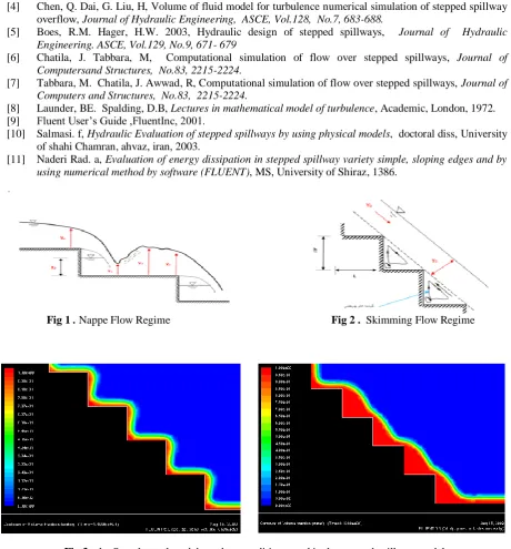
2.1.1.1 NAPPE FLOW REGIME: The flow, that which free jet, Collision of the upper step, to lower step. This
type of flow, occurs in low Discharge and high-tall steps. (Fig 1.)
2.1.1.2 SKIMMING FLOW REGIME: In the Skimming Flow Regime, steps act such as big coarseness against the flow. (Fig 2.)
2.1.1.3 TRANSITIONAL FLOW REGIME: If the crossing flow over the stepped spillways with slop and Arbitrary number of steps , at low Discharge a stat is falling, Gradually, then Discharge is increased, a case is observed, at the boundary between two Flow the Skimming and Nappe and the conversion threshold is, to Skimming Flow Regime, that this type of flow, is called transitional flow regime
2.2 THE GOVERNING EQUATIONS FOR THE FLOW
The incompressible fluid flow, continuity equation and momentum equation is expressed as follows: ∂ui
∂x j (1)
(2) ∂pui
∂t +
∂
∂xj pujui = − ∂p ∂xi+
∂
∂xj μ+μt ∂ui ∂xj+
𝜕𝑢𝑗 ∂xi
In which (t) is time, (ui) velocity component, (xi) coordinates component, (ρ) the density, (μ) the dynamic viscosity, (μt) the turbulent viscosity, (p') is the pressure corrected , is obtained the following equations.
(3)
p′ = p +2ρk
3
In which (P) is the pressure and (K) is the kinetic energy of perturbation. Also K and ε equations are expressed as follows:
(4) ∂(ρk)
∂t +
∂(uik) ∂xi =
∂ ∂xi (μ+
μt σk)
∂k
∂xi + G +ρε
(5) ∂(ρε)
∂t +
∂(uiε) ∂xi =
∂ ∂xi (μ+
μt σε)
∂ε ∂xi + C1ε
ε
KG − C2ερ ε2 K
In which (μt) is the turbulence viscosity by (k) kinetic energy of turbulence and (ε) the rate of energy dissipation of turbulence is obtained from the following relationshipship
(6) μt=ρcμk2
ε
In which Cμ = 0.09 is experimental constant. Prandtl Turbulence numbers for K and ε respectively include,the σk = 1.0 , σε= 1.3 , C1ε=1.44 , C2ε= 1092 are constants equation ε. generation turbulence kinetic energy G, in resulting average velocity gradient, is defined as follow.
(8) ∂ui
∂xj
G =μT= ∂ui ∂xj +
∂uj ∂xi
2.3 VOLUME OF FLUID MODEL (VOF)
Volume of Fluid model (VOF) by Hirt and Nichols was suggested in 1981. That to determine common surface of two fluid phases has been considered in many hydrodynamic issues. also In The hydraulic phenomena,free surface flow, is very important in solution of flow field. Various methods are used in determine the free surface, That,are different relative to prevailing view of solving the flow field. In VOF method, for each a component volume of cell is solved a differential equation, which ultimately amount component volume of fluid is determined in each cell. In flow field with the fixed network, is determined determine free surface based on the view O'Leary toward flow. Equations formulation are basis on fluid volume models (VOF), based on the fact that two or more fluid phases that together they are not mixed together. The purpose of this model is to find, the interface between phases in different parts of domain. Although the basis of this theoretical model, is polyphase flows, but, VOF model is not a polyphase model. For example, in the case of two-phase gas (air) and water, a series momentum equations between the two phases is be shared. For each fluid phase is added to the modeI in fact, one variable, into Solving process and this variable, is the component volume of fluid in each of calculated cells, So that the sum volume of fluid component in a cell is equal to the unit. In the case two phases water and air component volume of fluid water or air can be considered as a added variable.if aw is a component volume of water. Then, component volume of air, is equal to.
(7)
aa= 1 − 𝑎w
volume component. In other words and in the general case, if, the component volume of q-th phase existing in computational cell, is shown by 𝛼q,then is represented following three modes.
αq= 0, corresponding to the case ,that cell is lack the q-th fluid.
αq= 1, corresponding to the case, that computational cell, is full the q-th fluid.
0 <αq< 1, corresponding to the case ,that computational cell, is, containing surface subscription between the q-th fluid, with one or more other fluids.
III. ISSUE DESCRIPTION AND NUMERICAL SOLUTION
3.1 BOUNDARY CONDITIONS GRIDDED OF MODELS
In this research, For mesh Models made, are used the regular mesh with triangular elements. In Figure (3), we can see how the mesh and Boundary conditions used for the models stepped spillway models. For numerical analysis, has been used the FLUENT software, that works based on finite volume method. in Figure (3). in Fig (3), (A): the velocity inlet boundary condition, (B): the air inlet boundary conditions, that form zero pressure, (C): the air inlet boundary conditions, that form zero pressure, (D) : the walls boundary conditions, (F): is the outlet boundary conditions, which is considered to be zero pressure and, (E): the surface flow profile initial conditions, is in stepped spillway.
3.2 THE GEOMETRIC CHARACTERISTICS OF MODELS
In total,for the stepped spillways, has been considered, 2 Group Model With 5th and 10th steps, That each group has been considered for the three Discharge in per units width (q) 0.025, 0.039, 0.057 (m2/s) and critical flow depth (yc) 0.40, 0.054,0.069 (m). In all models, is steps height, in 5 stepped models, 0.085m and for models with 10 steps, steps height of 0.1722 meters. For total models, were considered spillway height, equal and 1m. The slope of spillway for all models is 45 degree and the spillway crest is climactic. (Table 1.)
3.3 NUMERICAL ANALYSIS STEPPED SPILLWAY
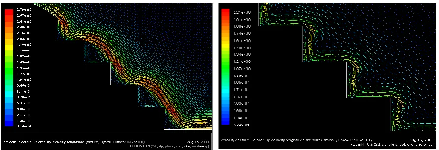
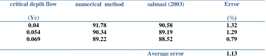
In Table (2) the results related to numerical analysis, is presented in each 2 groups stepped spillway (6 models). In this table, observed the types of flow and calculated the rate of energy dissipation from numerical analysis, can bee seen for each of the models. In Figures of (4), (5) and (6), can be observed, the Flow profiles formed in the models. The flow surface profiles obtained from the numerical analysis , which have surface flat almost and low curvature, ,is called continuous flow (Skimming Flow) and the flows, which have Deformation in the surface flow, is considered Transation Flow and the flows which have falling jet down over Steps are named nappe Flow. In Figure (7), (8) and (9), can be observed, the velocity field shaped in the models.
3.4 COMPARISON BETWEEN THE RESULTS NUMERICAL ANALYSIS WITH EXPERIMENTAL RELATIONSHIPSHIPS:
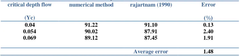
In tables (3), (4) and (5), respectively, Can be observed Comparison the numerical results with experimental relationshipships, of the researchers such as, Salmasi (2003), chanson (1994) and Rajartnam (1990). In this tables, which is relate to the Group 1 (with 5 steps) of the numerical analysis can be investigated to availabel errors between the numerical method and experimental method. Comparison of the numerical method shows for calculating the energy dissipation in simple stepped spillway groups one with Salmasies experimental relationships in 2003, whit three discharge per unit width 0.025, 0.039 and 0.057 (m2/s), respectively, 1.32%, 1.29% and 0.79% and with chanson experimental relationships (1994),respectively, 1.76%, 0.40% and 0.54% error and with Rajartnams experimental relationships (1990), respectively, 0.46% , 0.94% and 0.29% error and the results has suitable error, That from this Viewpoint Shows the proximity of numerical solution with experimental work.
In tables (6), (7) and (8), respectively, Can be observed Comparison the numerical results with experimental relationshipships, of the researchers such as, Salmasi (2003), chanson (1994) and Rajartnam (1990). In this tables, which is relate to the Group 2 (with 10 steps) of the numerical analysis can be investigated to availabel errors between the numerical method and experimental method. Comparison of the numerical method shows for calculating the energy dissipation in simple stepped spillway groups one with Salmasies experimental relationships in 2003, in three discharge per unit width 0.025, 0.039 and 0.057 (m2/s), respectively, 2.29%, 0.20% and 0.27% and with chanson experimental relationships (1994), respectively, 1.88%, 1.44% and 0.97% error and with Rajartnams experimental relationships (1990), respectively, 0.13% , 2.40% and 1.91% error and again the results has suitable error, That from this Viewpoint Shows the proximity of numerical solution with experimental work.
energy dissipation. Figure (12) shows the variation of discharge in the simple stepped spillway, that ,by increasing flow discharge is reduced energy dissipatio.
In the forms, tables and diagrams are provided to compare the results obtained from the variation of different parameters numerically and compared these changes with results obtained from empirical relations for models made, has shown that near diagrams in numerical models with experimental models, indicating nearby and agreement between the numerical model in the compared with experimental models.
3.5 COMPARE AND DIAGNOSIS TYPE OF FLOW NUMERICAL METHOD WITH EXPERIMENTAL RELATIONSHIPS:
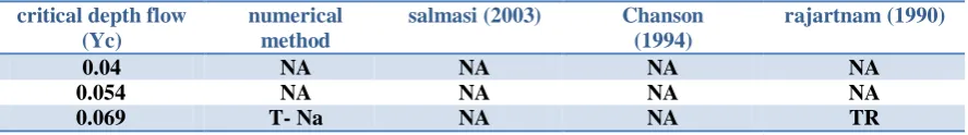
In tables (9), (10) and (11), respectively, Can be observed Comparison the numerical results with experimental relationshipships,of the researchers such as, Salmasi (2003), Rajartnam (1999) and chanson (1994) for the simple stepped spillway. In this table, which is related to the groups 1 and 2 of numerical analysis, can be observed, the results of numerical methods compatible well with other the researchers methods. In following table, (TR) representative the Transition flow, (SK) representative the Skimming flow and (NA) as agent representative is Nappe flow.
IV. CONCLUSIONS
In this research, firstly, was checked the effective factors on energy dissipation in types of stepped spillways, by means numerical method, which in previous researches, were checked by means numerically, Then, impact of each of these factors (the number of step), rate of Discharge, height and width of the step and ...),as can be observed in the rate of energy dissipation. In this research, the results obtained from the calculation of energy dissipation and diagnosis type of flow in Types of stepped spillways, by means numerical methods were compared, by the experimental relationships. the results obtained from of this research The effective factors on energy dissipation in types of stepped spillway can help designers for design better and more economical. The results of this part of the research, are compliance with the experimental results Salmasi (1382), Chanson (1994) and Rajartnam (1990). The error percentage obtained in the calculated energy dissipation by numerical method, in the compared with the experimental relationships can be caused of the calculated water surface in the numerical model, which, is considered in relationships to calculate the energy dissipation. Therefore we can, with the more accurate measurement of calculation water surface in the numerical model or use deep water after hydraulic jump (due to the air outlet in this area) in relationships to energy dissipation, to obtained more accurate results and minimize errors.
The numerical analysis in this research ,can be reached the following results.
According to the results obtained from the numerical models and comparison with experimental models, and their low error can be used, low cost and speed of numerical methods such as Fluent numerical model, instead of expensive testing in, hydraulic structures.
The energy loss in the stepped spillways,is further,the smooth spillways.
Increased Discharge over stepped spillways, causing increased velocity flow,and converting flow to the skimming flow, and ultimately, will reduce the energy dissipation.
in the stepped spillways Increasing the number of steps (height steps reduction) when height Dam is fixed, causing the surface steps sooner to be submerged below the surface water, and resulting, Causing, is reducing energy dissipation.
in the stepped spillways whit the Increasing height of steps, will cause the, spillways,act as vertical slope breakers, and with the creation, nappe flow, will increase energy dissipation.
Decrease of slope, in stepped spillways, is causes increases energy dissipation.
Increase the length of steps in a from that are fixed the height of steps and or the height of steps are equals, causes the crossing flow, larger surface (coarse), have for to contact their face, and Consequently,causes is increased of the energy dissipation.
The results that, numerical method is present to detection type of flow in the stepped spillways, to relationships, experimental, Salmasi in 1382, Chanson in 1994, and Rajartnam in 1990 are presented, for detection type of flow is fully compliance.
V. RESOURCES AND REFERENCES
[1] Christodoulou, G.C, Energy dissipation on stepped spillway, Journal of Hydraulic Engineering, ASCE, Vol.119, No.5, 644-649.
[2] Chamani, M.R. and Rajaratnam, N, Jet flow on stepped spillways, Journal of Hydraulic ASCE, Engineering. Vol.120, No.2, 254-259
[4] Chen, Q. Dai, G. Liu, H, Volume of fluid model for turbulencenumerical simulation of stepped spillway overflow, Journal of Hydraulic Engineering, ASCE, Vol.128, No.7,683-688.
[5] Boes, R.M. Hager, H.W. 2003, Hydraulic design of stepped spillways, Journal of Hydraulic Engineering. ASCE, Vol.129, No.9, 671- 679
[6] Chatila, J. Tabbara, M, Computational simulation of flow over stepped spillways, Journal of Computersand Structures, No.83, 2215-2224. [7] Tabbara, M. Chatila, J. Awwad, R, Computational simulation of flow over stepped spillways, Journal of
Computers and Structures, No.83, 2215-2224.
[8] Launder, BE. Spalding, D.B, Lectures in mathematical model of turbulence, Academic, London, 1972. [9] Fluent User’s Guide ,FluentInc, 2001. [10] Salmasi. f, Hydraulic Evaluation of stepped spillways by using physical models, doctoral diss, University
of shahi Chamran, ahvaz, iran, 2003.
[11] Naderi Rad. a, Evaluation of energy dissipation in stepped spillway variety simple, sloping edges and by using numerical method by software (FLUENT), MS, University of Shiraz, 1386.
Fig 1 . Nappe Flow Regime Fig 2 . Skimming Flow Regime
Fig 3 . the Sample mesh and boundary conditions used in the stepped spillway models Fig 4 . nappe Flow profiles in stepped spillway model
Fig 8 . velocity vectors of Transation flow in stepped spillway Fig 7 . velocity vectors of nappe flow in stepped spillway
Fig 9 . velocity vectors of skimming flow (Continuous) in stepped spillway model Fig 10 . Diagram, changes, of step height, in stepped spillway
Fig 11 . Diagram, changes the number of step in and changes of step length, in simple stepped spillway stepped spillway
91.78
90.34
89.27 91.22
90.02
89.12 88.5
89 89.5 90 90.5 91 91.5 92
0 0.05 0.1
ΔΗ
/Η
t
Yc (m)
L & h=0.1722m
L & h=0.085m 91.78
90.34
89.27 91.22
90.02
89.12 88.5
89 89.5 90 90.5 91 91.5 92
0 0.02 0.04 0.06
ΔΗ
/Η
t
YC(m)
Fig 12 . Diagram, changes of discharge, in simple stepped spillway Table 1 . Specifications of geometric, stepped spillway models
Group Q (m3/s) q (m2/s) yc (m) H (m) L (m) Hdam (m) N Slope ( Degree ) 1
0.01236 0.025 0.040 0.1722 0.1722 1.00 5 45
0.01952 0.039 0.054 0.1722 0.1722 1.00 5 45
0.0282 0.057 0.069 0.1722 0.1722 1.00 5 45
2
0.01236 0.025 0.040 0.085 0.085 1.00 10 45
0.01952 0.039 0.054 0.085 0.085 1.00 10 45
0 .0282 0.057 0.069 0.085 0.085 1.00 10 45
Table 2 . the Results numerical analysis of stepped spillway
Group Q (m3/s) q (m2/s) yc (m) h (m) L (m) Hdam (m) N Type of flow ∆𝐇 𝐇𝐭 % Slope ( Degree ) 1
0.01236 0.025 0.040 0.1722 0.1722 1.00 5 NA 91.78 45 0.01952 0.039 0.054 0.1722 0.1722 1.00 5 NA 90.34 45 0.0282 0.057 0.069 0.1722 0.1722 1.00 5 NA 89.22 45 2
0.01236 0.025 0.040 0.085 0.085 1.00 10 T-S 91.22 45 0.01952 0.039 0.054 0.085 0.085 1.00 10 T-S 90.02 45 0 .0282 0.057 0.069 0.085 0.085 1.00 10 T-S 89.12 45 Table 3 . Comparison of results, numerical and experimental methods, the simple stepped spillway, Group 1,
with Salmasi (2003)
critical depth flow
(Yc)
numerical method
( 𝚫𝐇 𝐇𝐭 % ) salmasi (2003) ( 𝚫𝑯 𝑯𝒕 % ) Error ( % )
0.04 91.78 90.58 1.32
0.054 90.34 89.19 1.29
0.069 89.22 88.52 0.79
Average error 1.13
91.78 90.34 89.27 91.22 90.02 89.12 88.5 89 89.5 90 90.5 91 91.5 92
0 0.01 0.02 0.03 0.04 0.05 0.06
Table 4 . Comparison of results, numerical and experimental methods, the simple stepped spillway, Group 1, with chanson (1994)
critical depth flow
(Yc)
numerical method
( 𝚫𝐇 𝐇𝐭 % )
chanson (1994)
( 𝚫𝐇 𝐇𝐭 % )
Error
(
%
)
0.04 91.78 90.19 1.76
0.054 90.34 89.98 0.40
0.069 89.22 89.70 -0.54
Average error 0.54
Table 5 . Comparison of results, numerical and experimental methods, the simple stepped spillway, Group 1, with rajartnam (1990)
critical depth flow
(Yc)
numerical method
( 𝚫𝑯 𝑯𝒕 % )
rajartnam (1990)
( 𝚫𝑯 𝑯𝒕 % )
Error
(
%
)
0.04 91.78 92.20 -0.46
0.054 90.34 89.50 0.94
0.069 89.22 89.48 -0.29
Average error 0.06
Table 6 . Comparison of results, numerical and experimental methods,the simple stepped spillway, Group 2, with salmasi (2003)
critical depth flow
(Yc)
numerical method
( 𝚫𝑯 𝑯𝒕 % )
salmasi (2003)
( 𝚫𝑯 𝑯𝒕 % )
Error
(
%
)
0.04 91.22 93.36 -2.29
0.054 90.02 89.84 0.20
0.069 89.12 89.36 -0.27
Average error -0.47
Table 7 . Comparison of results, numerical and experimental methods, the simple stepped spillway, Group 2, with chanson (1994)
critical depth flow
(Yc)
numerical method
( 𝚫𝑯 𝑯𝒕 % )
chanson (1994)
( 𝚫𝑯 𝑯𝒕 % )
Error
(
%
)
0.04 91.22 89.54 1.88
0.054 90.02 88.74 1.44
0.069 89.12 88.26 0.97
Average error 1.43
Table 8 . Comparison of results, numerical and experimental methods, the simple stepped spillway, Group 2, with rajartnam (1990)
critical depth flow
(Yc)
numerical method
( 𝚫𝑯 𝑯𝒕 % )
rajartnam (1990)
( 𝚫𝑯 𝑯𝒕 % )
Error
(
%
)
0.04 91.22 91.10 0.13
0.054 90.02 87.91 2.40
0.069 89.12 87.45 1.91
Table 9 . Comparison of results ,numerical method and experimental method, in simple stepped spillway, Group 1
rajartnam (1990) Chanson
(1994) salmasi (2003)
numerical method critical depth flow
(Yc)
TR NA
NA NA
0.04
SK TR
NA NA
0.054
SK NA
NA NA
0.069
Table 10 . Comparison of results, numerical method and experimental method, in simple stepped spillway, Group 2
rajartnam (1990) Chanson
(1994) salmasi (2003)
numerical method critical depth flow
(Yc)
NA NA
NA NA
0.04
NA NA
NA NA
0.054
TR NA
NA T- Na