IJSRSET162667 | Received : 08 Nov 2017 | Accepted : 20 Nov 2017 | November-December-2017 [(3)8: 203-209]
© 2017 IJSRSET | Volume 3 | Issue 8 | Print ISSN: 2395-1990 | Online ISSN : 2394-4099 Themed Section: Engineering and Technology
203
3D Reconstruction and Visualization : A Comparison between
2D, 3D CT Images
Pranav R. Mathapati
*1, Dr. Anilkumar N. Holambe
2, Prof. Sushilkumar N. Holambe
2 *1M.E. Student, CSE Department, TPCT COE Osmanabad,Maharashtra, India
2HOD, CSE Department TPCT’s COE, Osmanabad,
Maharashtra, India
3PG-Co-ordinator TPCT’s COE, Osmanabad,
Maharashtra, India
ABSTRACT
In this paper, three-dimensional (3D) reconstruction and visualization of several 2D CT images based on MATLAB were investigated. The 3D visualization of CT images will provide the realistic 3D environment; which increases the efficiency of diagnosis and treatment in medicine. Here, the marching cubes algorithm was used for surface rendering and volume rendering. The splitting-box algorithm presented here which reduces the number of polygonal chains by adapting their size to the shape of the surface. The resulting polygonal chains offer a wide spectrum for representing the contour surface. An exact representation is achieved by a new type of generic patches calculated from the polygonal chains. Approximations of different quality may be obtained by combining the algorithm generating the patches with simple triangulations. Finally, 3D reconstruction of 2D CT images was done by using MATLABprogramme.
Keywords: Marching-cubes algorithm, 3D Construction, MATLAB, MRI images.
I.
INTRODUCTION
Surface rendering is a means of extracting meaningful and intuitive information from 3D data sets. This is achieved by converting the volume data into a surface representation using an extraction step and then using conventional computer graphics techniques to render the surface. The surface extraction process is very important and several techniques have been developed (Kaufman 1990).
Modern medical three-dimensional reconstruction is a branch of the scientific computing visualization technology, which is not only the theoretical innovation, but also important application in clinic diagnosing and medical jurisprudences. Anatomical structures can be segmented and identified as a stack of intersections with a number of parallel planes, corresponding to the 3D images slices. However, if the shape and morphology of the object is to be comprehended, too much imagination is left to the doctor. After image segmentation and reconstruction, the structure should be visualized and further manipulated in a more realistic way, which can improve the accuracy and validity in medical diagnosis.
Visualization of three-dimensional scalar fields, commonly called volume rendering, is an area that have seen. Since the developments from early 1980s, the nature of the data is such that the interior can be rendered as well as the surfaces bounding the object. Volume rendering techniques concentrate on visualizing internal features of choice, and surfaces, at the same time. Volume rendering is a large field within scientific visualization. While most of the efforts have been geared towards medical imaging, some of the methods can just as well be used for similarly constructed scalar fields obtained from other sources. Many different basic theories from a wide array of engineering fields and Physics are combined under the name volume rendering.
II.
BACKGROUND
volume rendering, is Ray casting. A method whose roots are in its modern incarnations can be traced back to Blinn, and then refined by Levoy. As the name suggests, it works by casting rays into a volume of data and then sample each ray along intervals. Its main advantage is that no intermediate geometry is produced during the process, thus minimizing aliasing. Approaches taking the opposite route by exploiting intermediate geometry for increased rendering speed include Shear-warp. The last few years has seen revitalization within the field with the arrival of programmable consumer graphics cards. The majority of software based approaches cannot produce interactive frame rates, but by using consumer graphics cards, most implementations can achieve good frame rates. This cheap and fast hardware has generated a number of new techniques, most notably. New and groundbreaking techniques are currently being developed and many have been released continuously during the past year. This trend will most likely continue as the hardware matures.
The development of GPU3 ray-casting over the past five years has led to flexible and fast hardware accelerated direct volume renderers. The popularity of GPU ray casting is thanks to its easy and straightforward implementation on nowadays GPUs as well as the great flexibility and adaptability of the core ray-casting algorithm to a specific problem set.
Several recent works deal with enhancing the visual and spatial perception of the anatomy from the 3D data set by advanced DVR, many based on GPU ray-casting. Kruger et al. propose Clear View for segmentation free, real-time, focus and context (F+C) visualization of 3D data. Clear View draws the attention of the viewer to the focus zone, in which the important features are embedded. The transparency of the surrounding context layers is modulated based on context layer curvatures properties or distance to the focus layer. Viola et al. presented importance driven rendering of volumes based on cut always allowing fully automatic focus and context renderings. Burns et al. extend importance driven volume rendering with contextual cutaway views and combine 2D ultrasound and 3D CT image data based on importance. Beyer et al. present a very sophisticated volume renderer, based on GPU ray-casting, for planning in neurosurgery. The renderer supports concurrent visualization of multimodal three-dimensional image, functional and segmented image
data, skull peeling, and skin and bone incision removal at interactive frame rates. Kratz et al. present their results for the integration of a hardware accelerated volume renderer into a virtual reality environment for medical diagnosis and education. The presented methods and techniques are closely related to our work. However the renderer is integrated within a virtual reality environment. Thus, no fusion of real and virtual data is performed and important augmented reality problems like interaction of real and virtual objects are not addressed.
F+C rendering for medical augmented reality, has been proposed in recent work by Bichlmeier et al. However was never fully realized using the GPU with the same degree of quality and performance as in the field of computer graphics. The presented methods are limited to rendering polygonal surface data, extracted by time consuming segmentation from the volume data set. Although the relevant anatomy and structures can be depicted, the approach suffers from lack of real volumetric visualization of medical image data. Important and standard medical visualization modes are impossible to achieve with these technique, i.e. Maximum Intensity Projection (MIP) and volume rendering of soft tissue. Another limitation is that the visualization is static and fixed to the time of mesh generation. Despite these drawbacks, the proposed video ghosting technique of the skin surface is promising as it enables a natural integration of the focus zone into the real video images.
the surface is manipulate e.g. rotated, there is no need to regenerate the surface. But this approach faces both space and time problems because of the large number of triangles generated by MC. For example, a 3D surface constructed from a typical high resolution volume data set of requires718 964 triangles, and these triangles need 25 MB memory for storage (each triangle requires 36bytes). In addition, the large number of triangles implies that more time is needed for the rendering. Because of these problems, it is difficult to use MC for interactive applications in 3D visualization. This is a serious problem in an application area such as medical visualization. Recently, Turk (1992) uses a re-triangulation technique that introduces new points onto a polygonal mesh, and then discards the old points to create a new mesh to reduce the number of triangles representing the given surface. Schroeder et al. (1992) use an approach of vertex removal and local re-triangulation for simplifying polygonal models. They remove vertices that are within a pre specified tolerance of a plane that approximates the surface near vertex. Their method also identifies sharp edges and sharp corners and makes sure such features are retained in order to better represent the original data. Both methods post-process the triangulated surface generated by MC. More recently, Muller and Stark (1993) propose a method which adaptively generates the surface i.e. adapts the size of triangles to the shape of surface. The problem with their method is that certain big objects could be ignored. This is because the method does not check the value of any sample point within a box or sub box. Their method also suffers from the crack problem.
III.
DESIGN & IMPLIMENTATION
Adaptive Marching Cubes:
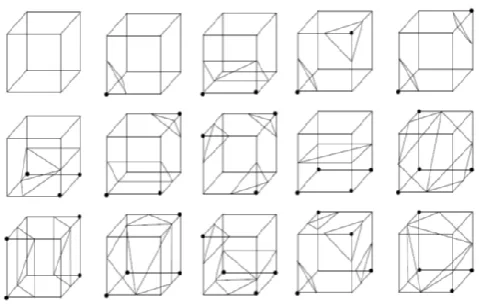
We briefly summarize the MC algorithm here in order to simplify the presentation of our algorithm. Marching cubes is a surface rendering algorithm that converts a volumetric data set into polygonal is valued (user-specified) surface consisting of triangles whose vertices are on the edges of the voxels (unit cubes) of the cuberille. The values of grid points and linear interpolation are used to determine where the valued surface intersects an edge of a voxel. The various configurations are shown in Figure 2.2, where a grid point that is marked indicates its value being above the threshold. While there are possible configurations, there are only 15 shown in Figure 2.2. This is because some
configurations are equivalent with respect to certain operations. First, the number can be reduced to 128 by assuming the two configurations are equivalent if marked grid points and unmarked grid points are switched. This means that we only have to consider cases where there are four or fewer marked grid points. Further reduction to 15 cases shown is possible by equivalence due to rotations.
A grid point that is marked indicates its value being above the threshold. While there are possible configurations, there are only 15 shown in Figure 1 this is because some configurations are equivalent with respect to certain operations. First, the number can be reduced to 128 by assuming the two configurations are equivalent if marked grid points and unmarked grid points are switched. This means that we only have to consider cases where there are four or fewer marked grid points. Further reduction to 15 cases shown is possible by equivalence due to rotations.
Basic AMC Strategy:
Assume that the volumetric data set size is, where (it’s easy to generalize AMC for an arbitrary size data set). As we mentioned in section 1.0, the basic strategy in AMC is to adjust the shape of the approximating surface based on the curvature of the actual surface within a cube. Initially, we partition the volumetric data set into cubes with equal size of, which we call initial cubes, where , and then use the MC surface configuration approach described in (Lorensen and Cline 1987) to triangulate the cubes, considering only the values of the 8 vertices of cubes. Then we recursively partition these cubes into Figure 1 Configurations of triangulated cubes.28 = 256.
The most important distinction is between structured and unstructured data since they often require different visualization methods, for example, shear-warp is a common technique used for structured data while projected tetrahedral is used for unstructured data. One should keep in mind also that these categorizations are not used to the letter by researchers.
The big driving force within the volume rendering field is without a doubt medical imaging. Medical scanners such as MR (magnetic resonance) measure three-dimensional space as a structured three-three-dimensional grid, and this has led researchers to focus mostly on volume rendering techniques based on structured, rectilinear grids. The grids are often called slices.
It should be noted that voxels can be defined in two different ways: It can be considered to be a cube formed by four neighboring grid points in two different slices and the whole voxel is covered by one single data value interpolated from all eight grid points. This definition is sometimes used in older publications.
Figure 1: Configuration of Triangulated Cubes
As with any rendering model, a mathematical model must first be defined in order to be able to create an image with volume rendering. The data can be density values for instance, and these need to somehow be mapped to optical properties. Depending on how realistic the final image must be, the model can include a number of physical properties, such as emission, absorption, reflection, scattering of light and occlusion of light. Today, the most common optical model used in volume rendering was developed by Blinn, and was later improved by Kajiya. Blinn initially developed the model so that he could render objects defined as volume densities with photo realism. He was specifically interested in rendering clouds and the rings of Saturn.
One of the unique features of directs volume rendering is the lack of actual surfaces. This is completely different to traditional computer graphics where polygonal or other types of surfaces with material properties are used. Instead of surfaces, Blinn regarded the density values within the data volume as small spherical particles. The particles scatter and attenuate light depending on their density.
According to Siegel et.al evaluating the 3.6 integral analytically on a computer is very difficult even though it can be done under certain circumstances. Computers in general are however much better suited to solve problems numerically. This calls for discrete version which can approximate the volume rendering integral. These approximations were commonly made by a Riemann sum. The viewing ray is divided it into equally long line segments. The absorption part can be rewritten;
Figure 2 : Basic AMC strategy explanation
The absorption part can be rewritten;
∫ ( )
∑
( )
∏ ( ( )
And the emission part becomes,
∫ ( ) ( ) ∑
Together the discrete version of the volume rendering integral is,
I(D)=IO∏ exp (γ(iΔx)Δx) + ∑ ciτi∏ exp(γ(iΔx)
Medical image data is a discrete three-dimensional regular data field, the value of each pixel as follows:
fi,j,k=f(xi,yj,zk),(i=1;Nx,j=1:Ny,k=1:Nz)
vertexes on the cube; for given threshold c0, the points which meet are called isosurface. If the value of the vertex greater than or equal to c0, the vertex (+) is located within the isosurface, otherwise the vertex (-) is located outside of isosurface. The cube is shown in figure 3.
Figure 3: Finding Isosurface
The Marching Cube Theory
The MC algorithm, which is originally proposed by Lorensen and Cline (1987), processes the 3D medical data in scan-line order. Since there are eight vertexes in each cube and two states (+ or -), there are only 28 = 256 ways the isosurface can intersect the cube, which can be reduced to 15patterns with the symmetry property, shown in figure 2.2 According to the 15 triangulated cubes, linear interpolation method is used to calculate the surface intersection x with cube edge:
x=i+(co-fi,j,k)|(fi+1,j,k-fi,j,k)
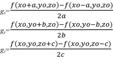
As the gradient vector is perpendicular to isosurface, the vertex normal vector can be expressed as:
gx=
( ) ( )
gy=
( ) ( )
gz=
( ) ( )
Polygon Strategy
In order to reduce the number of faces contributing to isosurface, polygons can be used to generate isosurface instead of triangles. The polygon strategy starts by finding all the isopoints lying on a cube according to step 3.1 and stores them into a list. The intersection on cube edge is up to one and each polygon edge is in the cube face, so each intersection isopoint has to belong to one polygon. The intersection edge has three cases: (a) v1 and v2 share a (+) vertex
(b) v1 and v2 share the edge with two (+) vertexes
©v1 and v2 share three (+) vertexes As shown in figure
Figure 4: Polygon strategy using isopoints
The intersection isopoints are ordered into a polygon according to the above cases, and then they are marked and stored in a list. The same procedure is repeated until every isopoint of the list is placed into a polygon. The implementation is described as follows:
Step1: find out all the isopoints lying on a cube, mark them as unmarked-isopoints and put them into a list; Step2: get an isopoint 1 from the list, make it current-isopoint and belong to polygon p; seek all points of according to step3;
Step3: get another isopoint v2 from the list, if v1 and v2are coplanar and meet
Step4: if the list has no unmarked-isopoint to meet step3, output p and return to step2; otherwise, if the list has no unmarked-isopoint, the cube has been processed, return tostep1 to deal with next cube. The polygon strategy does not require pre-defined configuration (Figure 3) and generates polygons which are equivalent to triangles in pre-defined configuration, so that produces fewer faces. It also can handle the ambiguity problem, avoiding the wrong topological links and the emergence of holes in isosurface.
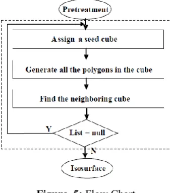
3D Reconstruction Algorithm
Figure 5: Flow Chart
This idea can be extended easily to the 3D case which we propose in this paper for AMC. Unfortunately, the problem is not so simple since AMC suffers from the crack problem encountered by all adaptive algorithms.
We now present the pseudo code of the AMC algorithm.
1. Divide up volume data set into initial cubes of equal size 2. for each initial cube
3. Call process cube(initial cube) 4. if cracks exist then
5. patch cracks
6. end if
7. end for
8. procedure process cube(cube)
9. if (cube contains a surface) then
10. Find intersections of the surface and cube edges ; 11. calculate intersection normal’s ;
12. if ( ( cube is of unit size ) or( any triangles with normal’s n0, n1 and n2, ARCCOS( )< for any) )
13. then
14. Output triangles ;
15. Store information for crack patching ; 16. else
17. Divide cube into 8 sub cubes
18. for each sub cube
19. Call process cube(subcube) 20. end for
21. end if 22. else
23. Store information for crack patching 24. end if
25. endprocess_cube
IV.
EXPERIMENTAL RESULTS
In order to evaluate the performance of proposed approach, real medical images of human skull MRI data sets with resolution of 256 × 256, from 27 slices, 1mm pitch are used. The experiment is executed in MATLAB under Windows8 on a PC with Core 2 Duo [email protected], 4GB of RAM, 160GB HD, and NVIDIA GeForce 8400M GS(256MB) graphics card, whose results obtained by the proposed approach, compared with the traditional method, are shown in following figure 6.1
Figure 6: MRI images
Following are the screenshots explaining 2-D to 3-D conversion of MRI images,
Figure 7: Loading MRI Images
Figure 9: Image after entering Iso value 5 Figure
Figure 10: Image after rotating 3-D Image in any direction
The results are satisfied. There is little different between the two methods. The reason why the mesh modal is white area in Figure 5(c) is that the generated faces are too small, which is also proved that the DMC method is feasible, because the maximum error is only 0.5 cube side lengths by midpoint instead of intersection, while the display devices often cannot meet the accuracy. The table1 shows the cost in time and space between the two methods on the comparison.
V.
CONCLUSION & FUTURE SCOPE
The proposed approach in this paper analyses the theory and shortcomings of MC algorithm, and then gives the details of the medical reconstruction. Experimental results illustrate that our method gives a great improvement on storage space and processing speed. The quality of modeling’s also achieved with satisfactory efforts. The significance of the approach in practical applications allowing real-time operations (e.g. rotation and scaling) and interactive performance with computer by less hardware cost. Future work should focus on the extraction of multi-organization sectional
image, which is formed by more than one single connected region.
The above algorithm can be improved for execution time in future also this can be made available on standalone system with hardware acceleration for the real time application.
VI.
REFERENCES
[1] Lars Kjelldahl, Beatriz Sousa Santos, ‘Visual
perception in computer graphics courses’, Computer &Graphics, (28), 2004, 451-456.
[2] R. R. Kothawale, R. M. Mohite, Advanced
Materials Research 1110, 2015, 218-221.
[3] Cline H E, Lorensen W E, ‘Marching Cube: A high
resolution 3D surface construction algorithm’, Computer Graphics, , 21 (4), 1987.
[4] R. M. Mohite, R. R. Kothawale, Indian Journal of
Chemistry 54A, 2015, 872-876.
[5] Cline H E, Lorensen W E, Ludke S. Two algorithms
for three-dimensional reconstruction oftomograms.
Med Phys, 15(3), 1988, 320~327.
[6] Montani C, Scateni R, Scopigno R. Discretized
marching cubes, Proceedings of visualization’
94,Washington, 1994, p281–7.
[7] Durst M J. Additional reference to marching cubes.
Computer Graphics, 22 (2), 1988, 72-73.
[8] J Wilhelms, AVanGelder. Topological
considerations in isosurface Generation. San Diego Workshop on Volume, Visualization, 24 (5), 1990, 79-86.
[9] R.M. Mohite, J.N. Ansari, A.S. Roy, R.R.
Kothawale, International Journal of Nanoscience,
15(1), 2016, 1650011.
[10] Digital Imaging and Communications in Medicine
(DICMO). National Electrical
ManufacturersAssociation, 1999.
[11] Tomas Akenine-Moller, Tomas Moller, and Eric
Haines, Real-time rendering, A. K. Peters,Ltd.2002.
[12] D. Bartz, M. Hauth, and K. Mueller, Advanced
Virtual Medicine: Techniques andApplications for
Virtual Endoscopy, MICCAI Tutorial T8, 2003.
[13] R. M. Mohite, R. R. Kothawale, International
Journal of Scientific Research, 3(12), 2014, 355-357.
[14] M.J Bentum, B.B.A. Lichtenbelt, and T. Malzbender,
Frequency analysis of gradi-ent estimators in
volume rendering, Tech. report, University of