R E S E A R C H
Open Access
Estimation of gait normality index based
on point clouds through deep auto-encoder
Trong-Nguyen Nguyen
1*and Jean Meunier
1Abstract
This paper proposes a method estimating an index that indicates human gait normality based on a sequence of 3D point clouds representing the walking motion of a subject. A cylinder-based histogram is extracted from each cloud to reduce the number of data dimensions as well as highlight gait-related characteristics. A model of deep neural network is finally formed from such histograms of normal gait patterns to provide gait normality indices supporting gait assessment tasks. The ability of our approach is demonstrated using a dataset of 9 different gait types performed by 9 subjects and two other datasets converted from mocap data. The experimental results are also compared with other related methods that process different input data types including silhouette, depth map, and skeleton as well as state-of-the-art deep learning approaches working on point cloud.
Keywords: Gait, Normality index, Auto-encoder, Deep network
1 Introduction
Gait normality index estimation is one of the most com-mon studied problems to support healthcare systems. Many researchers employed complex marker-based and multi-camera systems to acquire more details for gait analysis. One of their drawbacks is that they require spe-cific devices with high price and/or have high computa-tional cost. Therefore, some recent studies employed a single camera to deal with gait analysis problems. Depend-ing on the used sensors, the input of those methods is either subject’s silhouette or depth map. The former infor-mation has been used to propose numerous gait signa-tures such as motion history image (MHI) [9], gait energy image (GEI) [11], and active energy image (AEI) [17]. Each signature is a compression of a sequence of consecutive 2D silhouettes and is represented as a single grayscale or binary image. They were usually applied for the task of person identification. However, in the case of gait nor-mality index estimation, using only the gait signature is not enough. Nguyen et al. [20] employed MHI to estimate four-dimensional features. They processed each individ-ual silhouette as well as segmented each input sequence of frames into gait cycles where the temporal context
*Correspondence:[email protected]
1DIRO, University of Montreal, Pavillon André-Aisenstadt, 2920 chemin de la Tour, Montreal, H3T 1J4 Canada
was embedded in. The gait assessment was performed on each gait cycle using a one-class model that was trained with normal gait patterns, i.e., unsupervised learning. Bauckhage et al. [4] also proposed an approach detect-ing unusual movement. They put a camera to capture the frontal view of a walking subject. Each silhouette was encoded by a flexible lattice that followed a vector conver-sion of coordinates corresponding to a set of predefined control points. The temporal characteristic was then inte-grated into each feature vector by concatenating vectors of consecutive frames. Differently from [20], the gait normal-ity decision was determined based on a binary SVM where both normal and abnormal gait samples appeared in the training set. However, in many applications, using only a sequence of silhouettes as the input would lose important gait information because of the missing depth.
In order to deal with that limitation, depth sensors replaced color cameras in some studies. A popular device is the Kinect, which is provided by Microsoft with a low price and a SDK containing the functionality of
per-frame 3D human skeleton localization [29, 30]. Such
skeletons played the main role in some recent studies of gait-related problems such as pathological gait anal-ysis [8], gait recognition [16], and abnormal gait detec-tion [21]. These approaches, however, still have a draw-back since each skeleton is determined based on a depth frame. Concretely, self-occlusions in depth maps might
lead to unusual skeleton postures, and embedded gait characteristics would thus be deformed.
In this paper, we present an approach dealing with the problem of gait normality estimation. We focus on a setup of cheap equipments to capture the motion from differ-ent view points. We employ a time-of-flight (ToF) depth camera together with two mirrors so that the system can work in the manner of a collection of cameras while keep-ing the cost much lower than multi-camera systems [22]. A subject performs her/his walking gait on a treadmill at the center of the setup. A depth map captured by our setup is presented in Fig.1. As shown in the figure, there are 3 regions (highlighted with ellipses) corresponding to partial subject’s surfaces seen from different view points. A point cloud representing the subject can thus be easily formed as a combination of 3 collections of reprojected points (from 2D to 3D) including (a) the real cloud in the middle and (b) reflections (through mirror planes) of vir-tual clouds that are behind the two mirrors. An example of such reconstructed 3D point cloud is presented in Fig.2. More details on this reconstruction method are given in [22]. The input of our method is a sequence of these 3D point clouds that are formed based on consecutive depth frames captured by the depth camera. The output is gait normality indices provided by a model of normal walking postures. To our knowledge, this is the first work that per-forms gait normality index estimation on a sequence of 3D point clouds representing a walking person.
Our contributions are summarized as follows:
• Proposing a deep auto-encoder that learns common features of gait normality based on histograms of
Fig. 1A depth map captured by our setup that shows 3 devices including two mirrors and a treadmill where each subject performs her/his walking gait. Three collections of subject’s pixels are highlighted by ellipses
point clouds and a discussion on cloud-oriented deep networks for gait analysis
• Demonstrating the potential of point cloud in gait analysis problems compared to typical input data types such as skeleton, depth map, and silhouette
2 Proposed method
Our method consists of three main steps. First, a 2D histogram of each point cloud is formed to normalize the data dimension as well as highlight gait-related char-acteristics. Then, the second stage generates a model representing postures corresponding to normal walking gait based on a collection of 2D histograms. Finally, this model is used to compute a normality index for gait analysis.
2.1 Cylindrical histogram estimation
There are some inconveniences when performing gait assessment on 3D point clouds: (1) the number of points inside each cloud is not normalized, (2) such cloud may contain redundant information that are not useful for gait-related tasks, and (3) there may be some noises in each cloud, i.e., points reconstructed from depth values con-taining noise in the depth map. Therefore, each 3D point cloud is converted into a 2D histogram by fitting a cylin-der with equal sectors. It is worth noting that this step of normalization also plays an important role when working with neural networks since such models require inputs of fixed dimensions. Its axis coincides with the normal vec-tor of the treadmill surface and goes through the cloud’s centroid. Illustrations of the cylinder fitting and histogram formation are shown in Fig.3.
Let us notice that the coordinate system in that figure is flexible. The only constraint is that they-axis must be normal to the treadmill surface. The coordinate system in Fig.3is to show the relation between cylindrical sectors and their mapped elements in the corresponding 2D his-togram. Such arrangement of elements inside a histogram is to highlight the balance of human posture embedded in the point cloud. In other words, our cylindrical his-togram is considered as a smart projection of a 3D point cloud onto a frontal (or back) grid. The element values of each histogram are finally scaled to give a grayscale image of 256 levels. This representation is convenient for data range normalization and for storing. An exam-ple of grayscale histogram and the corresponding human posture is given in Fig.4.
2.2 Model of normal gait postures
Fig. 2The point cloud reconstructed from a depth map using the method [22]
sequence of posture assessments. An unsupervised learn-ing is appropriate since we are focuslearn-ing on estimatlearn-ing gait normality index. A model that is formed from a train-ing set containtrain-ing both normal and abnormal gaits may have a low generalization. The reason is that patterns of abnormal gaits would significantly affect the classi-fier because there are too numerous possible types of walking postures with abnormality in practical situations. Therefore, we attempt to create a model describing com-mon characteristics of normal gait postures. A typical way of performing this task is learning a vocabulary of code words extracted from histograms of normal gait. Recently, such approaches have demonstrated good per-formance on common problems such as content-based image retrieval [2,42] and image classification [3,40,41]. Another approach is the use of pretrained deep networks for feature extraction such as [27, 31]. These methods, however, are applied on natural images with an appropri-ate resolution, in which each code word is formed from
an image patch. Therefore, vocabulary learning is not suit-able to deal with our histograms of small size 16×16. Since deep learning has provided very good results in recent studies, we decide to employ such structures that can automatically determine useful features itself and work as a one-class classifier. The deep auto-encoder [26] is thus chosen in our approach to model normal gait postures.
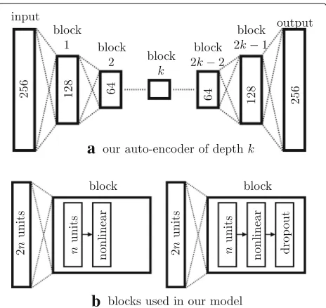
Our model structure is similar to a typical neural net-work but has some specific constrains. First, the model is a stack of blocks with the same layers inside. The only dif-ference between these blocks is the number of input and output connections. Each block contains a fully connected layer, a nonlinear activation layer, and an optional dropout layer. The dropout layer is considered to reduce the risk of overfitting [32]. We selected 3 popular activation func-tions including sigmoid, tanh, and leaky ReLU (rectified linear unit) for the middle (or last if no dropout) layer in each block. The original ReLU function is not considered
because it may cause the problem of dead neuron [18]
a
b
c
Fig. 4Example of 2D histogram estimated by fitting a cylinder onto a 3D point cloud:aposture,bgrayscale histogram, andcpseudo-color histogram for better visualization. The size of this histogram is 16×16
when embedded into a deep fully connected neural net-work where the learning rate is not small enough.
Let us consider a blocklwhere its fully connected layer is parametrized by weightsW(l)and biasesb(l), the output of anith unit given an inputx(l)is computed as
⎧ ⎪ ⎨ ⎪ ⎩
y(il)=Wi(l)x(l)+b(il) zi(l)=fy(il)
ˆ
zi(l)=Ui
p,Nx(l) ∗z(il)
(1)
wheref indicates one of the three mentioned activations,
N(x(l)) is the number of units connected from the pre-vious block, and U(p,n) is a function that produces n
binary values where p is the probability of zero ones.
The block output zˆ(l) is the input of the next block, i.e.,x(l+1)← ˆz(l).
The second constrain is that when the data is propa-gated from one block to the next, the number of dimen-sions is reduced by half. This property is reasonable since auto-encoders are to compress and highlight useful fea-tures inside the input. These two constrains are illustrated in Fig.5. Since we consider one of three activation func-tions including sigmoid, tanh, and leaky ReLU, there are thus 6 different structures that can be employed for con-structing our model. Notice that in the partial network of decoder, the number of units in a next block is doubled but the order of layers inside each block is the same. The auto-encoder structure in our work is symmetric, i.e., we stack k−1 blocks with increasing data dimension after usingkblocks to encode an input histogram. We use the termblock-level depth(or simplydepth) to indicate such value ofk, a model of depthkwill thus have 2k−1 hidden blocks. The input of our network is a vector of 256 ele-ments that is vectorized from each 16×16 histogram. The loss function used in our work is the mean squared error
(MSE) combined with a L2-regularization to prevent the model from overfitting:
L(H,Hˆ)= 1
n
n
i=1
Hi− ˆHi
2
2
256 +λ
l
W(l)2
2 (2)
where H andHˆ respectively denote a batch of ninput
vectorized histograms of 256 elements and their recon-struction, W(l) indicates weights of the fully connected layer in block l, and λ is the regularization rate that controls the effect ofWs on the total lossL.
a
b
2.3 Normality index
Since the input and output of our auto-encoder are the same in the training stage, we expect that the model can learn common characteristics embedded in normal walk-ing gait. We also expect that the loss of information in case of abnormal posture inputs will be significantly higher compared with normal gaits. The normality index is com-puted for each individual posture as the MSE loss between the input and output vectors of the same size, i.e.,
I(h)= 1
256h−M(h) 2
2 (3)
wherehis an input vectorized cylindrical histogram and
Mdenotes the model estimating a reconstruction from
h. The gait assessment can be performed with or
with-out considering the temporal factor depending on specific problems. Recent studies working on time series data (e.g., action recognition or video retrieval) embedded this fac-tor into their processing in various fashions such as by considering the variance among successive key frames [38], concatenating consecutive frames [35], or using spe-cific neural network layers [36]. In our work, we directly
measure a normality index given a sequence ofn
cylin-drical histograms by simply averaging their frame-level indices:
I(h1..n)= 1
n
n
i=1
I(hi) (4)
This measure is appropriate for the task of gait normal-ity index estimation because of the following reason. A sequence of walking postures can be considered as a hier-archy: it is a collection of walking cycles and each cycle is a group of poses. Unlike related tasks such as action classification or behavior understanding, walking move-ment tends to be periodic. Given an input sequence that is long enough to cover a number of gait cycles, the average of frame-level normality indices is expected to implicitly indicate the overall measure through the gait cycles.
The details of our model parameters and the ability of measuring gait normality index for distinguishing normal and abnormal walking gaits are shown in the next section.
3 Experiments 3.1 Dataset
Our approach was experimented on a dataset that includes normal walking gaits and 8 simulated abnormal gaits [19]. The abnormal gaits were created by embedding asymmetry into walking postures. Concretely, this task was performed by one of the following actions: (a) padding a sole with 3 possible heights (5/10/15 cm) under the left or right foot or (b) attaching a 4-kg weight to the left or right ankle. There are thus 8 possible walking gaits with anomaly. The normal and abnormal gaits were performed
by 9 volunteers using a Kinect 2. Each gait was repre-sented by a sequence of 1200 consecutive point clouds. They were formed by applying the method proposed in [22] at a frame rate of 13 fps. The speed of the tread-mill was set at 1.28 kph. Beside 3D point clouds, our data acquisition also captured corresponding skeletons and sil-houettes using existing functionalities in the Kinect SDK. These two data types were employed for a comparison between our method and two other related studies. In summary, the dataset contains 1200 point clouds, 1200 silhouettes, and 1200 skeletons for each gait type of a subject. Our experimental procedures involving human subjects were approved by the Institutional Review Board (IRB). The experiments focus on assessing the efficiency of the proposed models and demonstrating the potential of point cloud in gait normality index estimation com-pared with typical inputs such as skeleton, silhouette, and depth map.
The dataset was split into two sets according to the sug-gestion in [19]. The first one including gaits of 5 subjects was used in the training stage. The gaits of the 4 remaining subjects were tested to evaluate the ability of our trained models. The same split was also used in our experiments on related works in order to provide a comparison. Beside that data separation, the leave-one-out cross validation (on subject) was also considered to evaluate our method in a more general fashion.
3.2 Auto-encoder hyperparameters
This section presents our selection for typical hyperpa-rameters and the strategy for finding a reasonable value for the block-level depthkof our auto-encoder.
3.2.1 Typical hyperparameters
First, we consider the algorithm that performs the weight update after each iteration. We employed the RMSProp [33] since the learning rate is adaptively changed instead of being a constant value. An initial learning rate of 0.0001 was thus reasonable. The momentum that controls con-vergence speed was set to 0.9 according to the suggestion in [33].
Such selection of learning rate leads to the choice of the constant that affects the negative slope of the element-wise nonlinear activation leaky ReLU, i.e., α in the equationf(x) = 1(x < 0)(αx)+1(x ≥ 0)(x). This parameter was set to 0.1 in our model because a too small value (such as 0.01) still sometimes causes the problem of dead neuron.
Theλcoefficient controlling the L2-regularization was set to 0.25 after evaluating some randomized generating values. For the training process, we used a batch size of 512 and 800 epochs for each possible network without dropout layer. The number of epochs used for training the models with dropout was higher (1600 in our work) as suggested in [32]. The model weights were initialized
according to the method proposed by [10]. Many
tra-ditional auto-encoders initialized their weights based on greedy layer-wise pre-training [7,13]. Our model, how-ever, is considered as a typical deep neural network where the input is a hand-crafting feature, our selection of weight initialization is thus reasonable. The collection of such hyperparameters is summarized in Table1.
3.2.2 Depth determination
An important factor that is not considered in the pre-vious section is the block-level depth of network [i.e.,k
in Fig.5a]. This is the last parameter which needs to be determined in order to form a specific network structure. We selected an appropriate value using a cross-validation strategy applied on the training data consisting of gaits of 5 subjects.
Concretely, the cross-validation was performed with 5 folds, in which each one corresponds to the gaits of a subject. For each value k, we tested 6 networks [3 non-linear activations with/without dropout layer]. Since an auto-encoder is considered as a lossy compression, it is obvious that increasing the number of blocks will increase the loss, i.e., the distance between an input and its recon-structed image. Therefore, we need a more meaningful criterion for depth selection instead of simply perform-ing a loss comparison. Let us recall that our auto-encoder would be trained with the goal of modeling normal walk-ing gait, and the ability of providwalk-ing gait indices that can well distinguish normal and abnormal gaits is thus suit-able for assessing the optimal value ofk. For a problem of
Table 1Empirically selected hyperparameters in our auto-encoders
Training algorithm RMSProp
Loss function MSE
Initial learning rate 0.0001
λ(L2-regularization) 0.25
Momentum 0.9
Batch size 512
α(leaky ReLU) 0.1
Number of epochs (without dropout) 800
Number of epochs (with dropout) 1600
Dropout probability 0.3
Weight initialization Xavier [10]
binary decision, the area under curve (AUC) of a receiver operating characteristic (ROC) curve is an appropriate measurement and was used here.
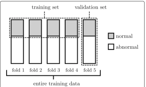
The stage of our fivefold cross-validation was performed as follows. Given a block-level depth value k0, we
con-structed 6 networks with 2k0 − 1 hidden blocks. Each
network would provide 5 applicable models since the training data was separated into 5 folds. Each model was trained with the normal gaits of 4 folds (4800 histograms) to get a collection of 10800 MSE loss values when eval-uating both normal and abnormal gaits (1200 and 9600 frames, respectively) of the remaining fold. A visualiza-tion of this separavisualiza-tion is shown in Fig.6. An AUC was finally estimated from such sequence of losses to repre-sent the model’s ability. Therefore, each of the 6 networks provided 5 AUCs in the stage of cross-validation given a specific depth. The mean AUC was calculated to represent the strength of each network for different depths in Fig.7. Notice that we did not consider the choice of block struc-ture, the cross-validation is just to find a reasonable depth for our auto-encoders.
According to Fig.7, assigning 4 as the network block-level depth is a good choice since it provided the highest mean AUC and a relatively small standard deviation (that can be considered as a stability criterion). Our final net-work was thus trained with 7 hidden blocks (i.e., depth of 4) with hyperparameters in Table1using all normal gaits in the training data. The overall architecture of our model can be represented as a sequence of blocks F128AD-F64AD-F32AD-F16AD-F32AD-F64AD-F128AD-F256, in
which FxAD indicates a block where F is a fully
con-nected layer that outputs x units, A is a nonlinear
activation (sigmoid, tanh, or leaky ReLU), and D is a dropout layer. When performing experiments on the models of non-dropout blocks, we simply set the dropout probability to 0.
Fig. 7AUCs estimated in our cross-validation stage with different choices of network depth
There were 6 possible auto-encoders corresponding to 6 block structures. They were employed independently in our evaluations. Our networks were implemented in Python with the use of TensorFlow [1].
3.3 Reimplementation of related methods
In order to provide a comparison with other related works that employed different input data types, we also per-formed experiments on skeletons and silhouettes using the methods proposed in [21] and [5], respectively. The recent study [23] was also considered since it represents features of interest as an intermediate between 2D (sil-houette) and 3D (depth map) information. Let us describe briefly these three approaches. The researchers in [21] directly employed the position of lower limb joints in skeletons provided by a Kinect to extract feature vectors representing the subject’s walking postures. A sequence of such vectors was then converted into a sequence of codewords using a clustering technique in order to sim-plify the feature space. The sequence was segmented into gait cycles by considering the change of distance between two feet. This step is necessary since the researchers focused on building a model of normal walking gait cycles using a specific Hidden Markov Model (HMM) struc-ture. The gait normality index was finally estimated for each input cycle as the log-likelihood provided by the trained HMM. Similarly to [21], the authors in [5] also performed the feature extraction on each silhouette using a lattice and embedded the temporal factor by concate-nating vectors estimated from a number of consecutive frames. A difference of this method from [21] and ours is that the researchers employed a supervised learning (binary support vector machine (SVM)) with two-class
training dataset to distinguish normal and abnormal walk-ing gaits. The method [23] estimated a gait-related score as a weighted sum of two scores corresponding to 2D and 3D information. Concretely, the researchers measured a LoPS (level of posture symmetry) score using a cross-correlation technique to describe the symmetry of 2D subject’s silhouette, and simultaneously employed a HMM to compute a PoI (point of interest) score according to key points determined from the corresponding depth map. A combination of those two scores provided good results in distinguishing between normal and abnormal walking gaits. In our experiments, we reimplemented a HMM of normal walking gait cycle for the study [21], a binary SVM
for [5], and a combination model of HMM and
cross-correlation for [23]. We also slightly modified the SVM to create a one-class SVM where the training stage only dealt with samples of normal gaits. These models and ours were trained and evaluated on the same dataset split but with different input types, i.e., point cloud, skeleton, and silhouette. Notice that depth maps for experimenting the study [23] were formed based on a projection of 3D point clouds according to the calibration information.
3.4 Evaluation metric
The ability of each proposed network was measured according to an equal error rate (EER) estimated based on the collection of MSE loss values. Since some related works attempted to embed the temporal context into their measurement, we also consider it by computing a sim-ple average EER over a short segment (length of 120 in our experiments) of histograms as well as over the entire sequence (i.e., length of 1200) corresponding to each walk-ing gait. Since we did not focus on selectwalk-ing the best block structure in this work, the average loss of the 6 networks (withk=4) was also computed. We also need to consider the measure for comparison since the three related works employed different quantities: the AUC for [21], the classi-fication accuracy for [5], and the EER for [23]. We selected the EER estimated from the ROC curve to represent the evaluation result of all models because this measure is related to both AUC and classification accuracy.
4 Results
The experimental results on the suggested data split (5 training subjects and 4 test subjects) and the leave-one-subject-out cross-validation are respectively presented in
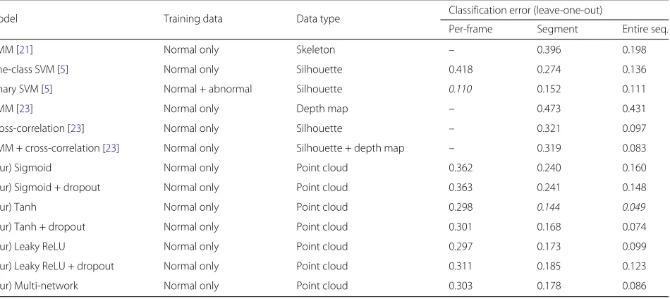
Tables 2 and 3. The last seven models are proposed in
our work, in which the termmulti-networkindicates the assessment of gait normality indices estimated as the aver-age of the losses resulting from the 6 other models. Notice that the notationsegment has different meanings: a sub-sequence of 120 histograms in our approach, a gait cycle that was automatically determined in [21], a per-frame
Table 2Classification errors (≈EERs) resulting from experiments on our auto-encoders and related studies with different data types
Model Training data Data type Classification error (4 test subjects)
†
Per-frame Segment Entire seq.
HMM [21] Normal only Skeleton - 0.335 0.250
One-class SVM [5] Normal only Silhouette 0.399 0.227 0.139
Binary SVM [5] Normal + abnormal Silhouette 0.104 0.157 0.139
HMM [23] Normal only Depth map - 0.396 0.281
Cross-correlation [23] Normal only Silhouette - 0.381 0.250
HMM + cross-correlation [23] Normal only Silhouette + depth map - 0.377 0.218
(Our) Sigmoid Normal only Point cloud 0.332 0.264 0.250
(Our) Sigmoid + dropout Normal only Point cloud 0.328 0.261 0.250
(Our) Tanh Normal only Point cloud 0.298 0.158 0.111
(Our) Tanh + dropout Normal only Point cloud 0.289 0.136 0.111
(Our) Leaky ReLU Normal only Point cloud 0.326 0.125 0.028
(Our) Leaky ReLU + dropout Normal only Point cloud 0.296 0.103 0.028
(Our) Multi-network Normal only Point cloud 0.288 0.125 0.083
†Our system was originally implemented in Mathematica [37]. The models without dropout provided better results compared with the ones performed by TensorFlow [1] in
this table. This may be because of the underlying algorithm implementation The italic values indicate the best results in different evaluations
recent frames in [5], and = 9 recent frames in [23]. These values were suggested by the authors in their orig-inal works. The termentire sequenceindicates EERs cal-culated based on the average loss over 1200 histograms in our method, lowest mean of log-likelihoods estimated on 3 consecutive walking cycles of a sequence in [21], alarm triggers in [5], and the average score in [23].
According to Tables 2and 3, employing the temporal
factor improved the accuracy in estimating the gait nor-mality index compared withper-frame(i.e., without con-sidering recent frames) estimation except for the binary SVM which is a supervised learning. Therefore, we should
focus only on the assessment performed onsegmentand
entire sequence. The classification errors almost always significantly decreased when the gait normality index was estimated over the input sequence instead of short seg-ments. Let us notice that our method measures the index of a sequence as a simple average of per-frame losses while the studies [5] and [21] used nonlinear computations, i.e., decisions respectively based on triggers and minimum 3-cycles means of log-likelihoods. In other words, those two methods assume that segment-based estimation pos-sibly contains noises (or outliers), a post-processing is thus required to provide a decision. Our method directly
Table 3Average classification errors (≈EERs) resulting from our leave-one-subject-out cross validation
Model Training data Data type Classification error (leave-one-out)
Per-frame Segment Entire seq.
HMM [21] Normal only Skeleton – 0.396 0.198
One-class SVM [5] Normal only Silhouette 0.418 0.274 0.136
Binary SVM [5] Normal + abnormal Silhouette 0.110 0.152 0.111
HMM [23] Normal only Depth map – 0.473 0.431
Cross-correlation [23] Normal only Silhouette – 0.321 0.097
HMM + cross-correlation [23] Normal only Silhouette + depth map – 0.319 0.083
(Our) Sigmoid Normal only Point cloud 0.362 0.240 0.160
(Our) Sigmoid + dropout Normal only Point cloud 0.363 0.241 0.148
(Our) Tanh Normal only Point cloud 0.298 0.144 0.049
(Our) Tanh + dropout Normal only Point cloud 0.301 0.168 0.074
(Our) Leaky ReLU Normal only Point cloud 0.297 0.173 0.099
(Our) Leaky ReLU + dropout Normal only Point cloud 0.311 0.185 0.123
(Our) Multi-network Normal only Point cloud 0.303 0.178 0.086
calculates the index considering every measured loss. There were also several noticeable factors related to the approach [23]. First, the combination of silhouette and depth map in [23] has a lack of generalization compared with our method. Since our dataset (with 8 abnormal gaits) is an extended version of the one in [23] (with-out gaits with a 4-kg weight attached to the left or right ankle), Table2 shows that the system [23] encountered difficulty in distinguishing those two additional abnormal gaits from normal ones. Another possible factor affect-ing the accuracy of method [23] is the size of training set (5 subjects in our experiments vs. 6 subjects in the origi-nal paper [23]). This was clearly demonstrated in Table3,
in which the method [23] provided good results when
there were 8 training subjects in each fold. It also showed that the generalization ability of our deep neural network is better compared with the combination of HMM and cross-correlation given a small training set.
In order to demonstrate the effect of the length of input walking postures, i.e. ,nin Eq. (4), we provide the assess-ment on various values of the temporal factor in Fig.8. These assessment results of default split and leave-one-out cross-validation schemes were respectively obtained from the models with leaky ReLU and tanh activations that provided best results in Tables 2 and 3. Figure 8 shows that the gait normality index estimation tent to be improved with the increasing number of successive postures. Therefore, estimating gait index on a pre-assigned sufficiently large number of frames is an appro-priate choice besides the typical consideration of walking gait cycle.
5 Comparison with deep learning models
With the fast development of deep learning, some net-works have been proposed to deal with 3D point cloud
Fig. 8EERs obtained when the gait normality index was estimated on different lengths of posture sequence
for popular objectives such as classification,
reconstruc-tion, and segmentation. We adaptively modified1 three
recent models including FoldingNet [39], PointNet [24], and RSNet [14] to obtain auto-encoder structures sup-porting the task of gait normality index estimation in the same fashion as ours. The former network is an auto-encoder, while the two others are segmentation networks. Details of the reimplementation and experimentation are as follows.
First, each model requires its inputs having the same shape, i.e., a fixed number of points. Therefore, we
employed random sampling [34] to downsample the
num-ber of points in each input cloud to 2048 for FoldingNet and PointNet and 4096 for RSNet. Second, we adapted the last layer and the objective function of PointNet and RSNet to obtain new architectures of point cloud recon-struction. Concretely, the number of channels in their last layer (corresponding to the number of segmentation categories) was replaced by the number of input chan-nels (i.e., 3 for the coordinates). The softmax loss was changed into MSE loss to force the models learning a way of reconstructing point position instead of perform-ing point classification. The Foldperform-ingNet originally uses Chamfer distance for the reconstruction since its input and output clouds have different sizes; we thus did not perform any modification on this model structure. The loss of these models were used to indicate the gait normal-ity index. In order to provide a comparison on processing time, we converted the framework of FoldingNet from Caffe [15] to TensorFlow [1].
Similarly to previous experiments, we evaluated the three networks using two schemes: the suggested data split and the leave-one-subject-out cross-validation. These models were respectively trained for 24000 and 9600 iterations with batch size of 1 for the two schemes. Notice that these numbers of iterations are just to evaluate the potential of models instead of guaranteeing a conver-gence. We also retrained our best networks (according to Tables2and3) in the same fashion for comparison. Since there was no classification model in this evaluation, we used AUC as the performance measure. The AUCs esti-mated on the gait indices outputted from all networks are shown in Fig.9. Notice that we consider only per-frame index.
Fig. 9AUCs estimated from our evaluation on deep learning models
Chamfer distance in gait index calculation is not signif-icantly affected by noise in the input cloud. Recall that there was no enhancement step performed on clouds in our experiments. On the contrary, PointNet and RSNet were directly designed for predicting point’s label instead of explicitly emphasizing informative hidden attributes to support the cloud reconstruction. Besides, the point neighborhood is determined using a small network in PointNet and a pooling layer in RSNet while FoldingNet directly considers the distance-based point graph. We believe that this is a reason for the large efficiency gap between FoldingNet and the two others in the task of cloud reconstruction.
A summary of single-cloud processing time correspond-ing to basic steps in our experiments is given in Table4. The evaluation was performed on a single GTX 1080 using Torch 0.4.1 (for RSNet) and TensorFlow 1.10.1 (for the others) with Python 3.5. It is obvious that FoldingNet takes very long times in both training and inference stages compared with our models. This is because we repre-sent each input cloud by a 16×16 matrix and this size does not increase during propagation in the network. On the contrary, FoldingNet operates on cloud coordi-nates together with the distance-based graph, performs multiple concatenations, and uses the costly Chamfer dis-tance as the loss function. It should also be noticed that
RSNet may be slightly slower when using TensorFlow since the study [28] reported that Torch is faster than TensorFlow.
6 Experiments on additional datasets
In addition to the dataset used for experiments in previous sections, we also performed some testing on two smaller datasets formed from mocap data. In detail, some mocap walking sequences including normal and looking-like-abnormal gaits (unbalance, hobble, skipping, swaggering)
were sampled from the CMU2and SFU3databases. These
mocap data were converted to point clouds by fitting a
3D model (created with MakeHuman4) and using the set
of 3D vertices as the point clouds. A summary of the two additional datasets used in this experiment is given in Table5.
In order to provide a comparison, we also reimple-mented two recent studies [6,25] that perform gait
anal-ysis on human movement. The method [25] decomposes
gait input signals into an ensemble of intrinsic mode func-tions to extract gait frequency properties and then ana-lyzes their association and inherent relations. The study [6] also considers periodical factors, but the gait features were manually estimated from 3D skeletons including average step length, mean gait cycle duration, and leg swing similarity. Both methods focus on efficient gait
Table 4Average processing time of basic operations in experimented models
Model Framework Preprocessing (using C++) Forward and backward (in training stage) Forward (in inference stage)
FoldingNet [39] TensorFlow 0.262(ms) 1.639 (s) 0.446 (s)
PointNet [24] TensorFlow 0.262(ms) 1.308 (s) 0.102 (s)
RSNet [14] Torch 0.311 (ms) 0.202 (s) 0.058 (s)
Our 6 models TensorFlow 1.126 (ms) 0.014(s) 0.002(s)
Table 5Number of frames and walking sequences in additional datasets
Dataset Training set (only normal gait) Test set Normal Abnormal
CMU 540 (5) 769 (8) 2224 ( 7)
SFU 1082 (5) 1295 (6) 3086 (13)
Each pair of valuesu(v)indicates a collection ofvsequences containing a total ofu frames
characteristics and employ simple learning algorithms for the assessment.
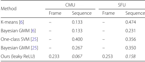
The experimental results (EER) are presented in Table6. It shows that our gait normality index was improved over a walking sequence instead of on each frame. Notice that these two datasets were selectively collected from mocap
databases focusing on action recognition. Table 6 also
shows that the cylindrical histogram can be appropriate for describing various gaits.
7 Discussion
First, let us explore in more detail the classification errors provided by the proposed auto-encoders. When embed-ding the temporal context into the estimation of gait normality index, the model which employed the leaky ReLU activation together with dropout layers provided the best results according to Table 2. In the leave-one-out cross-validation stage, replacing such combination by tanh activation gave the lowest classification errors. Therefore, more experiments as well as an extension of the dataset are needed to confirm the best block structure. However, the two tables show that using the tanh and/or leaky ReLU is preferred to sigmoid activation. In addition, the average of indices resulting from the 6 auto-encoders corresponding to 6 block structures (last row of Tables2 and3) demonstrated the potential of auto-encoder com-pared with the three other related methods.
Second, it is worth noting that our cylindrical histogram provides a good visual understanding (see Fig. 3) while intermediate features extracted from a cloud-oriented deep neural network would be much more difficult to
Table 6EERs obtained from experiments on two additional datasets
Method CMU SFU
Frame Sequence Frame Sequence
K-means [6] – 0.133 – 0.474
Bayesian GMM [6] – 0.133 – 0.231
One-class SVM [25] – 0.400 – 0.356
Bayesian GMM [25] – 0.267 – 0.350
Ours (leaky ReLU) 0.233 0.067 0.253 0.158
The two methods [6,25] are not adaptive to perform per-frame assessment The italic values indicate the best results
interpret. Therefore, our method is more appropriate for practical applications where users/operators are not familiar with the more difficult interpretation of interme-diate features in deep networks.
Another important factor is the coordinate system that is illustrated in Fig.3. A setting that does not satisfy this constraint might significantly affect the ability of extracted histograms in reasonably representing gait postures. In that case, a rigid transformation [12] is an appropriate solution to guarantee the constraint.
Finally, the local motion of body parts (e.g., limbs) is not explicitly considered in a sequence of cylindrical his-tograms. A further investigation of such local descriptions is expected to increase the applicability of the method to specific gait problems.
8 Conclusion
This paper proposes an approach that estimates the gait normality index based on a sequence of point clouds formed by a ToF depth camera and two mirrors. Using such system not only reduces the price of devices but also avoids the requirement of a synchronization protocol since the data acquisition is performed by only one cam-era. This work introduces a simple hand-crafting feature, cylindrical histogram, extracted from raw input clouds that efficiently represents characteristics of walking pos-tures. Auto-encoders with a specific block-level depth and various block structures are then employed to process such sequence of histograms, and the resulting losses are considered as gait normality indices. The efficiency of our method was demonstrated in the experiments using a dataset of 9 subjects with 9 different walking gaits. The quality of 3D point clouds provided by our setup was also highlighted in a comparison with other related works that employed different input data types (skeleton, silhouette, and depth map). Our method could be appropriate for many gait-related tasks such as assessing patient recovery after a lower limb surgery for instance.
In further works, elaborate experiments will be per-formed to select the block that is best appropriate with our model structure. Besides, sparsity constraints will be con-sidered to give visual understanding about characteristics embedded inside the cylindrical histograms that are useful for gait-related tasks. Finally, modeling specific patholog-ical gaits using our auto-encoders is also an interesting future study.
Endnotes
1The modification was performed on official public
resources of these studies. 2http://mocap.cs.cmu.edu/
3http://mocap.cs.sfu.ca/
Abbreviations
AUC: Area under curve; EER: Equal error rate; HMM: Hidden Markov model; MSE: Mean square error; ReLU: Rectified linear unit; ROC: Receiver operating characteristic; SVM: Support vector machine; ToF: Time-of-flight
Acknowledgements
We would like to thank Hoang Anh Nguyen (Aeva Inc., Mountain View, CA, USA) for useful discussions. This project used data adapted from (1) mocap.cs.cmu.edu created with funding from NSF EIA-0196217 and (2) mocap.cs.sfu.ca created with funding from NUS AcRF R-252-000-429-133 and SFU President’s Research Start-up Grant.
Funding
Financial support for this work was provided by the Natural Sciences and Engineering Research Council of Canada (NSERC) under Discovery Grant RGPIN-2015-05671.
Availability of data and materials
The dataset analyzed during the current study is available in the DIRO Vision lab repository,http://www-labs.iro.umontreal.ca/~labimage/GaitDataset Prepared (normalized) cylindrical histograms of size 16×16 are available at http://www-labs.iro.umontreal.ca/~labimage/GaitDataset/normhists.zip (unzip password:wUz7EcH9xG)
A Python implementation of this work will be available on Github upon the publication of the manuscript.
Two additional datasets used in our experiments are available at http://www-labs.iro.umontreal.ca/~labimage/AdditionalGaitSets.
Authors’ contributions
TNN carried out the work, designed the experiments, and drafted the manuscript. JM has supervised the work. All authors read and approved the final manuscript.
Competing interests
The authors declare that they have no competing interests.
Publisher’s Note
Springer Nature remains neutral with regard to jurisdictional claims in published maps and institutional affiliations.
Received: 7 September 2018 Accepted: 8 May 2019
References
1. M. Abadi, P. Barham, J. Chen, Z. Chen, A. Davis, J. Dean, M. Devin, S. Ghemawat, G. Irving, M. Isard, M. Kudlur, J. Levenberg, R. Monga, S. Moore, D. G. Murray, B. Steiner, P. Tucker, V. Vasudevan, P. Warden, M. Wicke, Y. Yu, X. Zheng, inProceedings of the 12th USENIX Conference on Operating Systems Design and Implementation, USENIX Association, Berkeley, CA, USA, OSDI’16. Tensorflow: a system for large-scale machine learning, (2016), pp. 265–283.http://dl.acm.org/citation.cfm?id=3026877.3026899 2. N. Ali, K. B. Bajwa, R. Sablatnig, S. A. Chatzichristofis, Z. Iqbal, M. Rashid,
H. A. Habib, A novel image retrieval based on visual words integration of sift and surf. PLoS ONE.11(6), 1–20 (2016).https://doi.org/10.1371/ journal.pone.0157428
3. N. Ali, B. Zafar, F. Riaz, S. Hanif Dar, N. Iqbal Ratyal, K. Bashir Bajwa, M. Kashif Iqbal, M. Sajid, A hybrid geometric spatial image representation for scene classification. PLoS ONE.13(9), 1–27 (2018).https://doi.org/10.1371/ journal.pone.0203339
4. C. Bauckhage, J. K. Tsotsos, F. E. Bunn, inThe 2nd Canadian Conference on Computer and Robot Vision (CRV’05). Detecting abnormal gait, (2005), pp. 282–288.https://doi.org/10.1109/CRV.2005.32
5. C. Bauckhage, J. K. Tsotsos, F. E. Bunn, Automatic detection of abnormal gait. Image Vis. Comput.27(1), 108–115 (2009)
6. S. Bei, Z. Zhen, Z. Xing, L. Taocheng, L. Qin, Movement disorder detection via adaptively fused gait analysis based on kinect sensors. IEEE Sensors J. 18(17), 7305–7314 (2018).https://doi.org/10.1109/JSEN.2018.2839732 7. Y. Bengio, P. Lamblin, D. Popovici, H. Larochelle, inProceedings of the 19th
International Conference on Neural Information Processing Systems, MIT Press, Cambridge, MA, USA, NIPS’06. Greedy layer-wise training of deep networks (MIT Press, Cambridge, MA, 2006), pp. 153–160
8. A. A. M. Bigy, K. Banitsas, A. Badii, J. Cosmas, in2015 7th International IEEE/EMBS Conference on Neural Engineering (NER). Recognition of postures and freezing of gait in Parkinson’s disease patients using Microsoft Kinect sensor, (2015), pp. 731–734.https://doi.org/10.1109/NER.2015.7146727 9. J. W. Davis,Hierarchical motion history images for recognizing human
motion. (Proceedings IEEE Workshop on Detection and Recognition of Events in Video, 2001), pp. 39–46
10. X. Glorot, Y. Bengio, inProceedings of the Thirteenth International Conference on Artificial Intelligence and Statistics, PMLR, Chia Laguna Resort, Sardinia, Italy, Proceedings of Machine Learning Research, vol. 9, ed. by Y.W. Teh, M. Titterington. Understanding the difficulty of training deep feedforward neural networks (PMLR, 2010), pp. 249–256
11. J. Han, B. Bhanu, Individual recognition using gait energy image. IEEE Trans. Pattern Anal. Mach. Intell.28(2), 316–322 (2006).https://doi.org/10. 1109/TPAMI.2006.38
12. R. Hartley, A. Zisserman,Multiple view geometry in computer vision. (Cambridge university press, New York, NY, 2003)
13. G. E. Hinton, S. Osindero, Y. W. Teh, A fast learning algorithm for deep belief nets. Neural Comput.18(7), 1527–1554 (2006).https://doi.org/10. 1162/neco.2006.18.7.1527
14. Q. Huang, W. Wang, U. Neumann, inThe IEEE Conference on Computer Vision and Pattern Recognition (CVPR). Recurrent slice networks for 3D segmentation of point clouds (IEEE, 2018)
15. Y. Jia, E. Shelhamer, J. Donahue, S. Karayev, J. Long, R. Girshick, S. Guadarrama, T. Darrell, inProceedings of the 22Nd ACM International Conference on Multimedia, ACM, New York, NY, USA, MM ’14. Caffe: Convolutional architecture for fast feature embedding, (2014), pp. 675–678.http://doi.acm.org/10.1145/2647868.2654889
16. S. Jiang, Y. Wang, Y. Zhang, J. Sun,Real Time Gait Recognition System Based on Kinect Skeleton Feature. (Springer International Publishing, Cham, 2015), pp. 46–57
17. Z. Lv, X. Xing, K. Wang, D. Guan, Class energy image analysis for video sensor-based gait recognition: a review. Sensors.15(1), 932–964 (2015). https://doi.org/10.3390/s150100932.http://www.mdpi.com/1424-8220/ 15/1/932
18. A. L. Maas, A. Y. Hannun, A. Y. Ng, inProc. ICML, vol 30. Rectifier nonlinearities improve neural network acoustic models (PMLR, 2013) 19. T. N. Nguyen, J. Meunier,Walking gait dataset: point clouds, skeletons and
silhouettes. Tech. Rep 1379, DIRO, University of Montreal, (2018).http://www. iro.umontreal.ca/~labimage/GaitDataset/dataset.pdf
20. T. N. Nguyen, H. H. Huynh, J. Meunier, inProceedings of the Fifth Symposium on Information and Communication Technology, ACM, New York, NY, USA, SoICT ’14. Extracting silhouette-based characteristics for human gait analysis using one camera, (2014), pp. 171–177.http://doi. acm.org/10.1145/2676585.2676612
21. T. N. Nguyen, H. H. Huynh, J. Meunier, Skeleton-based abnormal gait detection. Sensors.16(11), 1792 (2016).https://doi.org/10.3390/ s16111792.http://www.mdpi.com/1424-8220/16/11/1792 22. T. N. Nguyen, H. H. Huynh, J. Meunier, 3D reconstruction with
time-of-flight depth camera and multiple mirrors. IEEE Access.6, 38,106–38,114 (2018a).https://doi.org/10.1109/ACCESS.2018.2854262 23. T. N. Nguyen, H. H. Huynh, J. Meunier, in2018 IEEE EMBS International
Conference on Biomedical Health Informatics (BHI), Las Vegas, NV, USA. Assessment of gait normality using a depth camera and mirrors, (2018b), pp. 37–41.https://doi.org/10.1109/BHI.2018.8333364
24. C. R. Qi, H. Su, K. Mo, L. J. Guibas, inThe IEEE Conference on Computer Vision and Pattern Recognition (CVPR). Pointnet: deep learning on point sets for 3D classification and segmentation (IEEE, 2017)
25. P. Ren, S. Tang, F. Fang, L. Luo, L. Xu, M. L. Bringas-Vega, D. Yao, K. M. Kendrick, P. A. Valdes-Sosa, Gait rhythm fluctuation analysis for neurodegenerative diseases by empirical mode decomposition. IEEE Trans. Biomed. Eng. 64(1), 52–60 (2017).https://doi.org/10.1109/TBME.2016.2536438 26. T. N. Sainath, B. Kingsbury, B. Ramabhadran, in2012 IEEE International
Conference on Acoustics, Speech and Signal Processing (ICASSP). Auto-encoder bottleneck features using deep belief networks, (2012), pp. 4153–4156.https://doi.org/10.1109/ICASSP.2012.6288833 27. M. Sajid, N. Ali, S. H. Dar, N. Iqbal Ratyal, A. R. Butt, B. Zafar, T. Shafique,
M. J. A. Baig, I. Riaz, S. Baig, Data augmentation-assisted makeup-invariant face recognition. Math Probl. Eng.2018(2018)
learning software tools, (2016), pp. 99–104.https://doi.org/10.1109/CCBD. 2016.029
29. J. Shotton, A. Fitzgibbon, M. Cook, T. Sharp, M. Finocchio, R. Moore, A. Kipman, A. Blake, inCVPR, vol. 2011. Real-time human pose recognition in parts from single depth images, (2011), pp. 1297–1304.https://doi.org/10. 1109/CVPR.2011.5995316
30. J. Shotton, R. Girshick, A. Fitzgibbon, T. Sharp, M. Cook, M. Finocchio, R. Moore, P. Kohli, A. Criminisi, A. Kipman, A. Blake, Efficient human pose estimation from single depth images. IEEE Trans. Pattern Anal. Mach. Intell.35(12), 2821–2840 (2013).https://doi.org/10.1109/TPAMI.2012.241 31. S. Smeureanu, R. T. Ionescu, M. Popescu, B. Alexe, inImage Analysis and
Processing - ICIAP, vol. 2017, ed. by S. Battiato, G. Gallo, R. Schettini, and F. Stanco. Deep appearance features for abnormal behavior detection in video (Springer International Publishing, Cham, 2017), pp. 779–789 32. N. Srivastava, G. Hinton, A. Krizhevsky, I. Sutskever, R. Salakhutdinov, Dropout: a simple way to prevent neural networks from overfitting. J. Mach. Learn. Res.15, 1929–1958 (2014).http://jmlr.org/papers/v15/ srivastava14a.html
33. T. Tieleman, G. Hinton, Lecture 6.5-rmsprop: divide the gradient by a running average of its recent magnitude. COURSERA: Neural Netw. Mach. Learn.4(2), 26–31 (2012)
34. J. S. Vitter, Faster methods for random sampling. Commun ACM.27(7), 703–718 (1984).https://doi.org/10.1145/358105.893.http://doi.acm.org/ 10.1145/358105.893
35. B. Wang, X. Liu, K. Xia, K. Ramamohanarao, D. Tao,Random angular projection for fast nearest subspace search. (R. Hong, W. H. Cheng, T. Yamasaki, M. Wang, C. W. Ngo, eds.) (Springer International Publishing, Cham, 2018), pp. 15–26
36. X. Wang, L. Gao, P. Wang, X. Sun, X. Liu, Two-stream 3-D convNet fusion for action recognition in videos with arbitrary size and length. IEEE Trans. Multimed.20(3), 634–644 (2018).https://doi.org/10.1109/TMM.2017. 2749159
37. Wolfram Research Inc, Mathematica, Version 11.1. Champaign, IL, 2017 (2017).http://support.wolfram.com/kb/41360
38. K. Xia, Y. Ma, X. Liu, Y. Mu, L. Liu, inProceedings of the 25th ACM International Conference on Multimedia, ACM, New York, NY, USA, MM ’17. Temporal binary coding for large-scale video search, (2017), pp. 333–341. https://doi.org/10.1145/3123266.3123273
39. Y. Yang, C. Feng, Y. Shen, D. Tian, inThe IEEE Conference on Computer Vision and Pattern Recognition (CVPR). Foldingnet: point cloud auto-encoder via deep grid deformation (IEEE, 2018)
40. B. Zafar, R. Ashraf, N. Ali, M. Ahmed, S. Jabbar, S. A. Chatzichristofis, Image classification by addition of spatial information based on histograms of orthogonal vectors. PLOS ONE.13(6), 1–26 (2018a).https://doi.org/10. 1371/journal.pone.0198175
41. B. Zafar, R. Ashraf, N. Ali, M. Ahmed, S. Jabbar, K. Naseer, A. Ahmad, G. Jeon, Intelligent image classification-based on spatial weighted histograms of concentric circles. Comput. Sci. Inf. Syst.15(3), 615–633 (2018b).http://doiserbia.nb.rs/Article.aspx?id=1820-02141800025Z 42. B. Zafar, R. Ashraf, N. Ali, M. K. Iqbal, M. Sajid, S. H. Dar, N. I. Ratyal, A novel

![Fig. 2 The point cloud reconstructed from a depth map using the method [22]](https://thumb-us.123doks.com/thumbv2/123dok_us/874009.1584913/3.595.56.540.542.693/fig-point-cloud-reconstructed-depth-map-using-method.webp)