Combinatorial Species and Labelled Structures

(1)

University of Pennsylvania

ScholarlyCommons

Publicly Accessible Penn Dissertations

1-1-2014

Combinatorial Species and Labelled Structures

Brent Yorgey

University of Pennsylvania, [email protected]

Follow this and additional works at:http://repository.upenn.edu/edissertations

Part of theComputer Sciences Commons, and theMathematics Commons

This paper is posted at ScholarlyCommons.http://repository.upenn.edu/edissertations/1512

For more information, please [email protected].

Recommended Citation

(2)

Combinatorial Species and Labelled Structures

Abstract

The theory ofcombinatorial specieswas developed in

the 1980s as part of the mathematical subfield of enumerative

combinatorics, unifying and putting on a firmer theoretical basis a

collection of techniques centered aroundgenerating functions. The theory ofalgebraic data

typeswas developed, around the same time, in functional

programming languages such as Hope and Miranda, and is still used

today in languages such as Haskell, the ML family, and Scala. Despite

their disparate origins, the two theories have striking

similarities. In particular, both constitute algebraic frameworks in

which to construct structures of interest. Though the similarity has

not gone unnoticed, a link between combinatorial species and algebraic

data types has never been systematically explored. This dissertation

lays the theoretical groundwork for a precise—and, hopefully,

useful—bridge bewteen the two theories. One of the key

contributions is to port the theory of species from a classical,

untyped set theory to a constructive type theory. This porting process

is nontrivial, and involves fundamental issues related to equality and

finiteness; the recently developedhomotopy type theoryis put to good use formalizing these issues in a

satisfactory way. In conjunction with this port, species as general

functor categories are considered, systematically analyzing the

categorical properties necessary to define each standard species

operation. Another key contribution is to clarify the role of species

(3)

data structures, which have both labelled shapes and data associated

to the labels. Finally, some novel species variants are considered,

which may prove to be of use in explicitly modelling the memory layout

used to store labelled data structures.

Degree Type Dissertation

Degree Name

Doctor of Philosophy (PhD)

Graduate Group

Computer and Information Science

First Advisor

Stephanie C. Weirich

Keywords

combinatorics, programming languages, species, types

Subject Categories

(4)

COMBINATORIAL SPECIES AND

LABELLED STRUCTURES

Brent Abraham Yorgey

A DISSERTATION

in

Computer and Information Science

Presented to the Faculties of the University of Pennsylvania

in

Partial Fulfillment of the Requirements for the

Degree of Doctor of Philosophy

2014

Supervisor of Dissertation

Stephanie Weirich

Associate Professor of CIS

Graduate Group Chairperson

Lyle Ungar Professor of CIS

Dissertation Committee

Steve Zdancewic (Associate Professor of CIS; Committee Chair)

Jacques Carette (Associate Professor of Computer Science, McMaster University)

Benjamin Pierce (Professor of CIS)

(5)

COMBINATORIAL SPECIES AND LABELLED STRUCTURES COPYRIGHT

2014

Brent Abraham Yorgey

This work is licensed under a Creative Commons Attribution 4.0 International License. To view a copy of this license, visit

http://creativecommons.org/licenses/by/4.0/

The complete source code for this document is available from

(6)

ὅς ἐστιν εἰκὼν τοῦ θεοῦ τοῦ ἀοράτου,

πρωτότοκος πάσης κτίσεως,

ὅτι ἐν αὐτῷ ἐκτίσθη τὰ πάντα ἐν τοῖς οὐρανοῖς

καὶ ἐπὶ τῆς γῆς, τὰ ὁρατὰ καὶ τὰ ἀόρατα,

εἴτε θρόνοι εἴτε κυριότητες εἴτε ἀρχαὶ εἴτε

ἐξουσίαι· τὰ πάντα δι’ αὐτοῦ καὶ εἰς αὐτὸν

ἔκτισται·

καὶ αὐτός ἐστιν πρὸ πάντων

καὶ τὰ πάντα ἐν αὐτῷ συνέστηκεν,

καὶ αὐτός ἐστιν ἡ κεφαλὴ τοῦ σώματος τῆς

ἐκ-κλησίας·

ὅς ἐστιν ἀρχή,

πρωτότοκος ἐκ τῶν νεκρῶν, ἵνα γένηται ἐν πᾶσιν

αὐτὸς πρωτεύων,

ὅτι ἐν αὐτῷ εὐδόκησεν πᾶν τὸ πλήρωμα κατοικῆσαι

καὶ δι’ αὐτοῦ ἀποκαταλλάξαι τὰ πάντα εἰς

αὐτόν, εἰρηνοποιήσας διὰ τοῦ αἵματος τοῦ

σταυροῦ αὐτοῦ, εἴτε τὰ ἐπὶ τῆς γῆς εἴτε τὰ

ἐν τοῖς οὐρανοῖς·

(7)

Acknowledgments

I first thank Stephanie Weirich, who has been a wonderful advisor, despite the fact that we have fairly different interests and different approaches to research. She has always encouraged me to pursue my passions, even to the point of allowing me to take on a dissertation topic she knew very little about. Perhaps most importantly, she has done a masterful job getting me to actually graduate (no mean feat)—by turns encouraging and challenging me, each at the appropriate moment.

Jacques Carette has been an unofficial second advisor to me. Despite having plenty of “official” advisees also demanding his time and attention, he has generously taken the time to collaborate, give feedback and advice, and even twice to host me for a week of focused, face-to-face collaboration. This dissertation literally would not exist were it not for his academic and personal generosity, for which I will always be grateful.

My family has been, and continues to be, a constant source of joy and encour-agement. My wife and bestest friend Joyia, more than anyone else, is the one who encouraged me through the darkest points and convinced me to keep going. She has also sacrificed much in order to give me the time and space necessary to finish. My son Noah, too, has sacrificed—in ways he doesn’t even understand—while his daddy wrote a “very long story about computers and numbers”. But I could always count on him to cheer me up with tickle fights.

The other members of the Penn programming languages group—especially (though by no means limited to) Chris Casinghino, Richard Eisenberg, Nate Foster, Michael Greenberg, Peter-Michael Osera, Benjamin Pierce, Vilhelm Sj¨oberg, Daniel Wagner, and Steve Zdancewic—deserve a great deal of thanks for all their support over the years, through moral support and encouragement, critical feedback on papers and talks, enlightening discussions, and simply friendship. PL Club has been a wonder-fully collegial community in which to learn and work.

(8)

Yates, all of whom read early drafts of this dissertation and sent me typo reports as well as more substantial suggestions, greatly improving the final product. Thanks also to the anonymous MSFP and MFPS reviewers, whose feedback on submissions based on this material led to many substantial improvements to the technical content.

The diagrams community—particularly Daniel Bergey, Chris Chalmers, Allen

Gardner, Niklas Haas, Claude Heiland-Allen, Chris Mears, Jeff Rosenbluth, Carter Schonwald, Michael Sloan, Luite Stegeman, and Ryan Yates—has been a great source of joy to me during the long process of completing my PhD. Not only have they provided encouragement, camaraderie, and welcome distraction, but this dissertation itself is richer for their contributions todiagrams—many of the diagrams throughout this document make nontrivial use of features contributed by other members of the community. It has also been a particular joy to see the project continue humming along even during my virtual absence while writing.

It is staggering to consider the wealth of relationship accumulated during six years at City Church Philadelphia. I particularly thank Tuck and Stacy Bartholomew, Darren Bell, Dave and Katie Brindley, Zac and Joanna Brooks, Sara Cayless, Mike and Sonja Chen, Tim and Ruth Creber, Chris and Bonnie Currie, Ben Doane and Melissa McCarten, Megan and Ryan Dougherty, John Dyck, Brooke Fugate, Kevin Funderburk, Will and Margaret Kendall, Dick Landis, Colin and Lauren Marlowe, Drew and Susie Matter, Nick McAvoy, Chris and Sarah Miciek, Jeremy Millington, Cat Ricketts, Ben Smith, Josh and Kory Stamper, Ben Sykora and Beth Dyson, Matt Thanabalan and Carrie Lutjens, Gene and Laura Twilley, and Jackson Warren, all of whom, at various times and in various ways, have provided encouragement and support as I made my way through graduate school. It is certain that I have forgotten others who should also be on this list, and in any case it is not even clear where the list should stop!

I thank the Mustard Seed Foundation for their affirmation in selecting me as a Harvey Fellow, and for their support, both financially, and in helping me think through the integration of my faith and work.

A heartfelt thank you to the Williams College computer science department for the genuine care and support I have received as a visiting faculty member, and especially to Bill Lenhart for his generous gift of time in taking on most of the grungy legwork for CS 134. Beginning a new job, teaching two classes, and simultaneously completing a dissertation would be impossible even to contemplate were it not undertaken in such a supportive environment.

In Philadelphia, the Green Line Cafe, Lovers & Madmen, the Penn Graduate Student Center, and Van Pelt library—and in Williamstown, Tunnel City Coffee and the Schow science library—have all provided wonderfully conducive environments for focused writing sessions.

Last but certainly not least, a big thank you is due to Beeminder (http://

beeminder.com), and to its cofounders, Bethany Soule and Danny Reeves. The chance

(9)

vanish-ingly small, for the simple reason that a dissertation cannot be put off until a week before it is due. $145 for the motivation to write a dissertation is quite a steal; I owe the whole Beeminder team a round of beers!

Finally, my work has been supported by the National Science Foundation under the following grants:

• NSF 1218002, CCF-SHF Small: Beyond Algebraic Data Types: Combinatorial Species and Mathematically-Structured Programming

• NSF 1116620, CCF-SHF Small: Dependently-typed Haskell

• NSF 0910500, CCF-SHF Large: Trellys: Community-Based Design and Imple-mentation of a Dependently Typed Programming Language

and by the Defense Advanced Research Projects Agency under the following grant:

• DARPA Computer Science Study Panel Phase II.Machine-Checked Metatheory for Security-Oriented Languages.

Statement of contribution

(10)

ABSTRACT

COMBINATORIAL SPECIES AND LABELLED STRUCTURES Brent Abraham Yorgey

Stephanie Weirich

The theory of combinatorial species was developed in the 1980s as part of the mathematical subfield of enumerative combinatorics, unifying and putting on a firmer theoretical basis a collection of techniques centered aroundgenerating functions. The theory of algebraic data types was developed, around the same time, in functional programming languages such as Hope and Miranda, and is still used today in lan-guages such as Haskell, the ML family, and Scala. Despite their disparate origins, the two theories have striking similarities. In particular, both constitute algebraic frame-works in which to construct structures of interest. Though the similarity has not gone unnoticed, a link between combinatorial species and algebraic data types has never been systematically explored. This dissertation lays the theoretical groundwork for a precise—and, hopefully, useful—bridge bewteen the two theories. One of the key contributions is to port the theory of species from a classical, untyped set theory to a constructive type theory. This porting process is nontrivial, and involves fundamental issues related to equality and finiteness; the recently developedhomotopy type theory

(11)

(12)

List of Tables

(16)

List of Figures

1.1 An element ofSetX orSet/X . . . 20

1.2 The groupoidP . . . 29

2.1 The axiom of choice . . . 31

2.2 Representing a many-to-many relationship via a junction table . . . . 40

2.3 Eliminating >from both sides of an equivalence . . . 51

2.4 A path between inhabitants of UFin contains only triangles . . . 53

3.1 Representative labelled shapes . . . 61

3.2 The species L of lists . . . 61

3.3 The species B of binary trees . . . 62

3.4 The species E of sets . . . 62

3.5 An exampleMob-shape, drawn in four equivalent ways . . . 63

3.6 The species C of cycles . . . 63

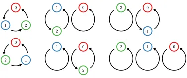
3.7 The species S of permutations . . . 64

3.8 An exampleEnd-shape . . . 64

3.9 Relabelling . . . 66

3.10 Inorder traversal is natural . . . 69

3.11 Permutations of size three . . . 70

3.12 Two permutations with the same form . . . 71

3.13 Two permutations with different forms . . . 71

3.14 S-forms of size 4 . . . 72

3.15 Lists and permutations on three labels . . . 73

3.16 The fundamental transform . . . 74

3.17 Correspondence between species and generating functions . . . 79

4.1 (B+L) 2 . . . 82

4.2 (B+B) 2 . . . 83

4.3 Four views on the Cartesian product B×L . . . 85

4.4 The unique E 5 shape . . . 86

4.5 Two views on the partitional species productB·L . . . 91

4.6 Permutation = fixpoints · derangement . . . 93

(17)

4.8 A Mat-shape of size 6 . . . 96

4.9 A Rect-shape of size 6 . . . 97

4.10 (X·X)-shapes . . . 99

4.11 Fin (m+n)−→∼ Fin m]Fin n−→∼ Fin m]Fin n −→∼ Fin (m+n) . . 103

4.12 Distinct choices of ϕthat result in identical permutations f . . . 103

4.13 Generic species composition . . . 107

4.14 An example (B◦L+)-shape . . . 107

4.15 The species Par of partitions . . . 107

4.16 An example (B×Par)-shape . . . 108

4.17 An example R-shape . . . 108

4.18 Example P-shapes . . . 109

4.19 An infinite family of (B◦L)-shapes of size 2 . . . 110

4.20 Indexed species product . . . 113

4.21 (C◦L)- and (L◦C)-forms of size 3 . . . 114

4.22 Internal Hom for composition . . . 116

4.23 An example B0-shape . . . 118

4.24 a0 ∼=E◦ A . . . 119

4.25 C0 ∼=L . . . 119

4.26 L0 ∼=L2 _{. . . .} ₁₁₉

4.27 The trivial up and down operators on E. . . 122

4.28 An up operator on L . . . 122

4.29 An up operator on B . . . 122

4.30 A down operator on C . . . 123

4.31 An example down operator on B, via stacking . . . 124

4.32 An example down operator on B, via promotion . . . 124

4.33 Species pointing . . . 125

4.34 An example B(K)_{-shape . . . .} ₁₂₆

4.35 “Currying” for partitional product of species . . . 127

4.36 “Currying” for arithmetic product of species . . . 129

4.37 A symmetry and a non-symmetry of a C-shape . . . 130

4.38 Isomorphism between L5/Z5 and C5 . . . 134

4.39 Isomorphism between L_>2/Z2 and E2·L . . . 134

4.40 The four molecular species of size 3 . . . 134

5.1 A typical copartial bijection . . . 141

5.2 Composition of copartial bijections . . . 142

5.3 Lifting a strictly copartial bijection . . . 147

5.4 B·E (bottom) is the prefix sum of B(top) . . . 150

5.5 A copartial species which loses information . . . 151

5.6 A two-sort species of binary trees . . . 153

5.7 A bicolored cycle . . . 153

(18)

(19)

This document is typeset in LA_{TEX using Computer Modern.}

It was edited usingemacs and stored using gitand github.com. The illustrations were produced with diagrams version 1.2 (http:

(20)

Chapter 0 Introduction

The theory of algebraic data types has had a profound impact on the practice of programming, especially in functional languages. The basic idea is that types can be built up algebraically from a small set of primitive types and combinators: a unit type, base types, sums (i.e. tagged unions), products (i.e. tupling), and recursion. Most languages with support for algebraic data types also add bells and whistles for convenience (such as labeled products and sums, convenient syntax for defining types as a “sum of products”, and pattern matching), but the basic idea remains unchanged.

For example, in Haskell [Marlow, 2010] we can define a type of binary trees with integer values stored in the leaves as follows:

dataTree=Leaf Int

| Branch Tree Tree

Algebraically, we can think of this as defining the type which is the least solution to the equationT =Int+T×T. This description says that aTreeis either anInt(tagged with Leaf) or a pair of two recursive occurrences of Trees(tagged with Branch).

This algebraic view of data types has many benefits. From a theoretical point of view, recursive algebraic data types can be interpreted as initial algebras (or

fi-nal coalgebras), which gives rise to an entire theory—both semantically elegant and

practical—of programming with recursive data structures viafolds and unfolds [Mei-jer et al., 1991, Gibbons, 2002]. A fold gives a principled way to compute a “summary value” from a data structure; dually, an unfold builds up a data structure from an initial “seed value”.

(21)

An algebraic view of data types also enables datatype-generic programming— writing functions that operate generically over values of any algebraic data type by examining its algebraic structure. For example, the following function (defined using Generic Haskell-like syntax [Hinze, 2000, Clarke et al., 2002]) finds the product of all the Int values contained in a value of any algebraic data type.

genProd {| Int |} i =i

genProd {| Sumt1 t2 |} (Inlx) =genProd {|t1 |} x

genProd {| Sumt1 t2 |} (Inrx) =genProd {|t2 |} x

genProd {| Prodt1 t2 |} (x,y) =genProd {|t1 |} x ∗genProd {| t2 |}y

genProd {| |} = 1

Datatype-generic programming is a powerful technique for reducing boilerplate, made possible by the algebraic view of data types, and supported by Haskell libraries and extensions [Jansson and Jeuring, 1997, L¨ammel and Jones, 2003, Cheney and Hinze, 2002, Weirich, 2006b,a].

The theory of combinatorial species has been similarly successful in the area of combinatorics. First introduced by Joyal [1981], it is a unified theory of

combinato-rial structures or shapes. Its immediate goal was to generalize the existing theory

of generating functions, a central tool in enumerative combinatorics (the branch of

mathematics concerned with counting abstract structures). More broadly, it intro-duced a framework— similar to algebraic data types—in which many combinatorial objects of interest could be constructed algebraically, and in which those algebraic descriptions can be used to reason about, manipulate, and derive properties of the combinatorial structures. The theory of species has been used to give elegant new proofs of classical results (for example, Cayley’s theorem giving the number of la-belled trees [Joyal, 1981]), and some new results as well (for example, a combinatorial interpretation and proof of Lagrange inversion [Bergeron et al., 1998, Chap. 3]).

Not only do the theory of algebraic data types and the theory of combinatorial species have a similar algebraic flavor in general, but the specific details are tantaliz-ingly parallel. For example, the species of binary parenthesizations (i.e. binary trees with data stored in the leaves) can be defined by the recursive species equation

P=X+P·X·P

which closely parallels the Haskell definition given above. The theory of functional programming languages has a long history of fruitful borrowing from pure mathemat-ics, as, for example, in the case of category theory; so the fruit seems ripe for picking in the case of combinatorial species.

(22)

The first to think about species specifically in the context of strongly typed func-tional programming were Carette and Uszkay [2008], who explored the potential of species as a framework to extend the usual notion of algebraic data types, and de-scribed some preliminary work adding species types to Haskell. More recently, Joachim Kock has done some theoretical work generalizing species, “container types”, and other notions of “extended data type” [Kock, 2012]. (Most interestingly, Kock’s work points to the central relevance of homotopy type theory [Univalent Foundations Pro-gram, 2013], which also emerges as a central player in this dissertation.)

However, there has still yet to be a comprehensive treatment of the precise con-nections between the theory of algebraic data types and the theory of combinatorial species. Bergeron et al. [1998] give a comprehensive treatment of the theory of species, but their book is written primarily from a mathematical point of view and is only tan-gentially concerned with issues of computation. It is also written in a style that makes it relatively inaccessible to researchers in the programming languages community—it assumes mathematical background that many PL researchers do not have.

The investigations in this dissertation, therefore, all arise from considering the central question, what is the connection between species and algebraic data types? A precise connection between the two would have exciting implications. It would allow taking much of the mathematical theory developed on the basis of species—for example, enumeration, exhaustive generation, and uniform random gen-eration of structures via Boltzmann sampling [Duchon et al., 2002, 2004, Flajolet et al., 2007, Roussel and Soria, 2009]—and applying it directly to algebraic data types. It is also possible that exploring the theory of species in an explicitly compu-tational setting will yield additional insights into the combinatorial setting.

There is also the promise of using species not just as a tool to understand and work with algebraic data types in better ways, but directly as a foundation upon which to build (a richer notion of) algebraic data types. This is particularly interesting due to the ability of the theory of species to talk about structures which do not correspond to algebraic data types in the usual sense—particularly structures which involve symmetry and sharing.

A data structure withsymmetry is one whose elements can be permuted in certain ways without affecting its identity. For example, permuting the elements of a bag always results in the same bag. Likewise, the elements of an ordered cycle may be cyclically permuted without affecting the cycle. By contrast, a typical binary tree structure has no symmetry: any permutation of the elements may result in a different tree. In fact, every structure of an algebraic data type has no symmetry, since every element in an algebraic structure can be uniquely identified by apath from the root of the structure to the element, so permuting the elements always results in an observably different value.

(23)

vertices. In general, such graphs may involve sharing, since multiple edges may refer to the same vertex, and vice versa.

In a language with first-class pointers, creating data structures with sharing is relatively easy, although writing correct programs that manipulate them may be another story. The same holds true for many languages without first-class pointers as well. Creating data structures with sharing in the heap is not difficult in Haskell, but it may be difficult or even impossible to express the programs that manipulate them.

For example, in the following code,

t =lett3 =Leaf 1

t2 =Brancht3 t3

t1 =Brancht2 t2

inBrancht1 t1

only one “Leaf” and three “Branch” structures will be allocated in memory. The tree

t2 will be shared in the nodet1, which will itself be shared in the nodet. Furthermore, in a lazy language such as Haskell, recursive “knot-tying” allows even cyclic structures to be created. For example,

nums = 1 : 2 : 3 :nums

actually creates a cycle of three numbers in memory.

Semantically, however, t is a tree, not a DAG, and nums is an infinite list, not a cycle. It is impossible to observe the sharing (without resorting to compiler-specific tricks [Gill, 2009]) in either of these examples. Even worse, applying standard func-tions such as fold and map destroys any sharing that might have been present and risks non-termination.

When programmers wish to work with “non-regular” data types involving sym-metry or sharing, they must instead work with suitable encodings of them as regular data types. For example, a bag may be represented as a list, or a graph as an ad-jacency matrix. However, this encoding puts extra burden on the programmer, both to ensure that invariants are maintained (e.g.that the adjacency matrix for an undi-rected graph is always symmetric) and that functions respect abstract structure (e.g.

any function on bags should give the same result when given permutations of the same elements as inputs).

The promise of using the theory of species as a foundation for data types is to be able to declare data types with symmetry and sharing, with built-in compiler support ensuring that working with such data types is “correct by construction”.

The grand vision of this research program, then, is to create and exploit a bridge between the theory of species and the theory and practice of programming languages. This dissertation represents just a first step in this larger program, laying the theo-retical groundwork necessary for its continued pursuit.

(24)

species is traditionally couched in untyped, classical set theory. To talk about data types, however, we want to work in typed and constructive foundations. Attempting to port species to a typed, constructive setting reveals many implicit assumptions that must be made explicit, as well as implicit uses of reasoning principles, such as the axiom of choice, which are incompatible with constructive foundations. The bulk of Chapter 2 defines the foundational groundwork which makes it possible to talk about species in a typed, constructive setting. In particular, the biggest issues are the difference between equality and isomorphism, and the constructive encoding of

finiteness (which is itself related to issues of equality and isomorphism). The recently

developedhomotopy type theory [Univalent Foundations Program, 2013] turns out to be exactly what is wanted to encode everything in a parsimonious way. The develop-ment of cardinal-finite sets in HoTT (along with a related concept I term “manifestly finite sets”) is novel, as is the development of HoTT analogues of the set-theoretic groupoids B and P.

Chapter 3 presents the theory of species itself. Much of the chapter is not novel in a technical sense. One of the main contributions of the chapter, instead, is simply to organize and present some relevant aspects of the theory for a functional programming audience. The existing species literature is almost entirely written for either hard-core combinatorialists or hard-core category theorists, and is not very accessible to the typical FP practitioner. Any attempt to make species relevant to computer scientists must therefore first address this accessibility gap.

Chapter 3 does also make a few novel technical contributions—for example, a char-acterization of equipotence in terms of manifestly finite sets, and a careful discussion of finite versus infinite families of structures and the relation to species composition. Most importantly, since Chapter 3 is already attempting to present at least two dif-ferent variants of species—the traditional definition based on set theory, and a novel variant based on homotopy type theory—it “bites the bullet” and considersarbitrary

functor categories, elucidating the categorical properties required to support each species operation. Although many individual species generalizations have been con-sidered in the past, this systematic consideration of the minimal features needed to support each operation is novel. This allows operations to be defined for whole classes of species-like things at once, and in some cases even allows for species-like things to be constructed in a modular way, by applying constructions known to preserve the required properties.

Chapter 5 goes on to explore particular species variants, evaluated through the framework of Chapter 3. Some variants have already been considered in the literature; others, such as the notion of copartial species considered in §5.2, are novel.

(25)

(26)

Chapter 1 Preliminaries

The main content of this dissertation builds upon a great deal of mathematical for-malism, particularly from set theory, category theory, and type theory. This chapter provides a brief overview of the necessary technical background, giving definitions, important intuitions, and references for further reading. Readers who merely need to fill in a few gaps may find such brief treatments sufficient; it is hoped that readers with less background will find it a useful framework and source of intuition for furthering their own learning.

1.1 Metavariable conventions and notation

A great many variables and named entities appear in this dissertation. To aid the reader’s comprehension, the following metavariable conventions are (mostly) adhered to:

• Metavariables f, g, h range over functions.

• Greek metavariables (especially α, β, σ, τ, φ, ψ) often range over bijections.

• Blackboard bold metavariables (e.g._C,_D,_E) range over categories, as do fraktur variables such as L and S.

• Names of specific categories use boldface (e.g.Set,Cat,Spe, B,P).

• Names of types or categories defined within homotopy type theory often use a calligraphic font (e.g. U, B, P, S).

• Metavariables A, B, C, range over arbitrary sets or types.

• Metavariables K, Lrange over finite sets or types.

(27)

• Names of specific species use a sans-serif font (e.g. X, E,L, C, B, R).

This dissertation also features a menagerie of notations to indicate “sameness”. To the outsider this must seem quite bewildering: how complicated can “sameness” be? Why would one ever need anything other than plain old equality (=)? On the other hand, to computer scientists and philosophers this should come as no surprise; equality turns out to be an incredibly subtle concept. Each of these symbols and their corresponding concepts will later be discussed in more depth; however, as an aid to the reader, we give a brief enumeration of them here, which can referred back to in case of confusion or forgetfulness.

• Equality (=) is the only notation which is overloaded. In the context of set theory, two sets A and B are equal, denoted A= B, when they have the same elements. In the context of homotopy type theory (§1.3), = denotespropositional

equality; A=B denotes the type of paths between the types A and B.

• In the context of set theory, the symbol := is used to introduce a definitional

equality; that is, x:=y is a definition of x rather than a proposition asserting the equality of two things.

• A −→∼ B denotes the set (or type) of bijections between sets (or types) A and

B. That is, if f : A −→∼ B then f is a function from A to B which possesses both a left and right inverse (denoted f−1_{). Note that in set theory, sets which}

are in bijection are typically not equal.

• In homotopy type theory, ≡ denotes judgmental equality, not to be confused with propositional equality (=). A fuller discussion of judgmental versus propo-sitional equality can be found in §1.3.2.

• The symbol :≡ also denotes a definitional equality, but in homotopy type the-ory rather than set thethe-ory. The symbol emphasizes the fact that a definition introduces a judgmental rather than a propositional equality.

• Again in homotopy type theory, A ' B denotes the equivalence of two types

A and B. Intuitively, equivalence can be thought of as a “very well-behaved” bijection,i.e. a bijection with some extra coherence conditions.

(28)

= (propositional) equality := definitional equality (set theory)

∼

−→ bijection

≡ judgmental equality :≡ definition equality (HoTT)

' equivalence

↔ logical equivalence

∼

= isomorphism

#

= species equipotence

≈ relabelling equivalence

∼ generic equivalence relation Table 1.1: “Sameness” relations

• An isomorphism is an invertible arrow in a category (§1.4), and is denoted by

A∼=B. The precise meaning of ∼= thus depends on the category under consid-eration. For example, in Set, the category of sets, isomorphisms are precisely bijections; in the category of pointed sets, isomorphisms are those bijections which preserve the distinguished element, and so on. Generally speaking, iso-morphisms can be thought of as “structure-preserving correspondences”.

• F =# G denotes the equipotence of two species, discussed in §3.3.

• f1 ≈ f2 denotes equivalence up to relabelling of species shapes, discussed in

§3.3.2.

• Finally,x∼yis often used in general to denote an equivalence relation (whichever one happens to be under consideration at the moment).

These notations are summarized in Table 1.1.

1.2 Set theory

A grasp of basic set theory (the element-of (∈) and subset (⊆) relations, intersec-tions (∩), unions (∪), and so on) is assumed. However, no background is assumed in

axiomatic set theory, or in particular its role as a foundation for mathematics. Issues

relating to axiomatic set theory are spelled out in detail as necessary (for example, the axiom of choice, in §2.1).

The set ofnatural numbers is denoted_N={0,1,2, . . .}. Thesize orcardinality of a finite setX, a natural number, is denoted #X(rather than the more traditional|X|, since that notation is used for another purpose; see§1.3). Given a natural numbern∈

N, the canonical size-n prefix of the natural numbers is denoted [n] ={0, . . . , n−1}.

(29)

• f(X) = {f(a)|a∈X} denotes the image ofX under f;

• f−1(b) ={a∈A|f(a) =b} denotes the preimage or fiber of b;

• f−1₍_Y_{) =} S

b∈Y f

−1₍_b_{) =} _{_a _∈ _A _|_f₍_a₎ _∈_Y_} _{likewise denotes the preimage of}

an entire set.

1.3 Homotopy type theory

Homotopy Type Theory (HoTT) is a relatively new variant of Martin-L¨of type

the-ory [Martin-L¨of, 1975, Martin-L¨of and Sambin, 1984] arising out of Vladimir Voevod-sky’s Univalent Foundations program [Voevodsky]. There is certainly not space to give a full description here; in any case, given the existence of the excellent HoTT Book [Univalent Foundations Program, 2013], such a description would be superflu-ous. Instead, it will suffice to give a brief description of the relevant parts of the theory, and explain the particular benefits of carrying out this work in the context of HoTT. Some particular results from the HoTT book are also reproduced as necessary, especially in§2.2. It is thus hoped that readers with no prior knowledge of HoTT will still be able to follow everything in this dissertation, at least at a high level, though a thorough understanding will probably require reference to the HoTT book.

Homotopy type theory, I will argue, is the right framework in which to carry out the work in this dissertation. Intuitively, this is because the theory of species is based centrally around groupoids and isomorphism—and these are topics central to homotopy type theory as well. In a sense, HoTT is what results when one begins with Martin-L¨of type theory (MLTT) and then takes the principle of equivalence (§1.3.4) very seriously, generalizing equality to isomorphism in a coherent way.

We begin our brief tour of HoTT with its syntax.

1.3.1 Terms and types

Some familiarity with dependent type theory on the part of the reader is assumed; we simply note quickly the standard features of HoTT, including:

• an empty type⊥, with no inhabitants;

• a unit type >, with inhabitant ?;

• sum types A+B, with constructors inl: A→ A+B and inr: B →A+B, as well as a caseconstruct for doing case analysis;

• dependent pairs (x :A)×B(x), with constructor h−,−i, and projection func-tions π1 : (x:A)×B(x)→A and π2 : (p: (x:A)×B(x))→B(π1 p);

(30)

• a hierarchy of type universes U0, U1, U2. . . .

Following standard practice, universe level subscripts will usually be omitted, withU

being understood to represent whatever universe level is appropriate in the context. HoTT also allows inductive definitions. For example,_N:U0denotes the

inductively-defined type of natural numbers, with constructors O:_N and S:_N→_N; we will use Arabic notation like 3 as a shorthand for S (S (S O)). We also have Fin : _N → U0,

which denotes the usual indexed type of finite sets, with constructors FO :Fin (S n) and FS :Fin n → Fin (S n). For example, one can check that Fin 3 has the three in-habitantsFO,FS FO, andFS(FS FO), and that in general Finn is the type-theoretic counterpart to [n] ={0,1, . . . , n−1}.

Although Agda notation [Norell, 2007] is mostly used in this dissertation for depen-dent pairs and functions, the traditional notationsP

x:AB(x) and

Q

x:AB(x) (instead

of (x:A)×B(x) and (x:A)→B(x), respectively) are sometimes used for emphasis. As usual, the abbreviations A×B and A → B denote non-dependent (i.e. when x

does not appear free in B) pair and function types, respectively.

1.3.2 Equality

HoTT distinguishes between two different types of equality:

• Judgmental equality, denoted x ≡ y, is defined via a collection of judgments

stating when things are equal to one another, and encompasses things like basic rules of computation. For example, the application of a lambda term to an argu-ment is judgargu-mentally equal to itsβ-reduction. Judgmental equality is reflexive, symmetric, and transitive as one would expect. Note, however, that judgmental equality is not reflected as a proposition in the logical interpretation of types, so it is not possible to reason about or to prove judgmental equalities internally to HoTT.

• Propositional equality. Given x, y :A, we writex=Ay for the proposition that

xand yare equal (at the typeA). The Asubscript may also be omitted,x=y, when it is clear from the context. Unlike judgmental equality, where x ≡ y is

a judgment, the propositional equality x=y is a type (or a proposition) whose

inhabitants are evidence orproofs of the equality ofxand y. Thus propositional equalities can be constructed and reasoned aboutwithin HoTT. Inhabitants of

x = y are often called paths from x to y; the intuition, taken from homotopy theory, is to think of paths between points in a topological space. The most important aspect of this intuition is that a path from a point x to a point

y does not witness the fact that x and y are literally the same point, but rather specifies aprocess for getting from one to the other. The analogue of this intuition in type theory is the fact that a path of typex=ycan havenontrivial

computational content specifying how to convert between x and y. There is

(31)

equality, and corresponds to a “trivial path with no computational content”; but, as the discussion above indicates, there can be other inhabitants of path types besides refl.

Note that it is possible (and often useful!) to have nontrivial higher-order paths,

i.e. paths between paths, paths between paths between paths, and so on.

1.3.3 Path induction

To make use of a path p : x = y, one may use the induction principle for paths, or

path induction. Path induction applies when trying to prove a statement of the form

∀x, y.(p:x=y)→P(x, y, p). (1.3.1) For the precise details of path induction, see the HoTT book [Univalent Foundations Program, 2013]. For this work, however, a simple intuition suffices: to prove 1.3.1 it suffices to assume that pisrefl and that xand y are literally the same,i.e. it suffices to prove ∀x. P(refl, x, x).

It is important to note that this doesnot imply all paths are equal torefl! It simply expresses that all paths must suitably “act like”refl, inasmuch as proving a statement holds for refl is enough to guarantee that it will hold for all paths, no matter how they are derived or what their computational content.

Path induction has some immediate consequences. First, it guarantees that func-tions are always functorial with respect to propositional equality. That is, ife:x=y

is a path between x and y, and f is a function of an appropriate type, then it is possible to construct a proof that f(x) = f(y) (or a suitable analogue in the case that f has a dependent type). Indeed, this is not hard to prove via path induc-tion: it suffices to show that one can construct a proof of f(x) = f(x) in the case that e is refl, which is easily done using refl again. Given e : x = y we also have

P(x)→P(y) for any type family P, called thetransport ofP(x) alongeand denoted

transportP₍_e_{), or simply} _e

∗ when P is clear from context. For example, if e : A = B

then transportX7→X×(X→C)(e) :A×(A→C)→B×(B →C). Transport also follows easily from path induction: it suffices to note thatid :P(x)→P(x) in the case when

e is refl.

1.3.4 Equivalence and univalence

(32)

The identity equivalence is denoted by id, and the composition of h:B 'C and

k : A ' B by h◦k : A ' C. As a notational shortcut, equivalences of type A ' B

can be used as functionsA →B where it does not cause confusion.

HoTT’s main novel feature is the univalence axiom, which states that equivalence is equivalent to propositional equality, that is, (A ' B) ' (A = B). One direction, (A = B) → (A ' B), follows easily by path induction. The interesting direction, which must be taken as an axiom, is ua : (A ' B) → (A = B). This formally encodes theprinciple of equivalence [nLab, 2014e], namely, that sensible properties of mathematical objects must be invariant under equivalence. Univalence, in conjunction with transport, implies that equivalent values are completely interchangeable.

Propositional equality thus takes on a meaning richer than the usual conception of equality. In particular, A=B does not mean that A and B are identical, but that they can be used interchangeably—and moreover, interchanging them may require some work, computationally speaking. Thus an equality e : A = B can have non-trivial computational content, particularly if it is the result of applying ua to some equivalence.

As of yet, univalence has no direct computational interpretation1, so using it to give a computational interpretation of species may seem suspect. However,uasatisfies theβ lawtransportX7→X₍_ua₍_f_{)) =}_f_{, so univalence introduces no computational}

prob-lems as long as applications ofuaare only ultimately used viatransport. In particular, sticking to this restricted usage ofuastill allows a convenient shorthand: packaging up an equivalence into a path and then transporting along that path results in “automat-ically” inserting the equivalence and its inverse in all the necessary places throughout the term. For example, let P(X) :≡ X ×(X → C) as in the example from the end of §1.3.3, and suppose e:A 'B, so ua e:A =B. Then transportP₍_ua₍_e_{)) :}_P₍_A₎_→

P(B), and in particulartransportP(ua(e))ha, gi=he(a), g◦e−1i, which can be derived mechanically by induction on the shape of P.

1.3.5 Propositions, sets, and

n

-types

As noted previously, it is possible to have arbitrary higher-order path structure: paths between paths, paths between paths between paths, and so on. This offers great flexibility but also introduces many complications. It is therefore useful to have a vocabulary for explicitly talking about types with limited higher-order structure.

Definition 1.3.1. A mere proposition, or (−1)-type, is a type for which any two inhabitants are propositionally equal.

The word “mere” is often used for emphasis (“mere proposition”) but is also sometimes dropped (“proposition”). Intuitively, the only interesting thing that can be said about a mere proposition is whether it is inhabited or not. Although it may

1_{Though as of this writing there seems to be some good progress on this front via the theory of}

(33)

have many syntactically different inhabitants, they are all equal and hence internally indistinguishable. Such types are called “propositions” since they model the way one usually thinks of propositions in, say, first-order logic. There is no value in distin-guishing the different possible proofs of a proposition; what counts is only whether or not the proposition is provable at all.

Definition 1.3.2. A type Ais a set, or 0-type, if there is (up to propositional equal-ity) at most one path between any two elements; that is, more formally, for any

x, y :A and p, q :x=y, there is a path p=q. Put another way, for any x, y :A, the type x=y is a proposition.

Standard inductive types such as_N, Fin n, and so on, are sets, although proving this takes a bit of work. Generally, one shows via induction that paths between elements of the type are equivalent to an indexed type given by⊥when the elements are different and > when they are the same; ⊥ and > are mere propositions and hence so is the type of paths. See the HoTT book for proofs in the particular case of _N, which can be adapted to other inductive types as well [Univalent Foundations Program, 2013,

§2.13, Example 3.1.4, §7.2].

As noted above, propositions and sets are also called, respectively, (−1)-types and 0-types. As these names suggest, there is an infinite hierarchy ofn-types (beginning at

n =−2 for historical reasons) which have no interesting higher-order path structure above level n. As an example of a 1-type, consider the type of all sets,

Set:≡(A:U)×isSet(A),

where isSet(A) :≡(x, y :A)→(p, q :x=y)→(p=q) is the proposition that A is a set. Given two elements A, B : Set it is not the case that all pathsA =B are equal; such paths correspond to bijections between A and B, and there may be many such bijections.

Note that isSet(A) itself is always a mere proposition for any typeA (see Lemma 3.3.5 in the HoTT book).

1.3.6 Higher inductive types

Another novel feature of HoTT (albeit one that is not yet fully understood) is the presence ofhigher inductive types (HITs). Standard inductive data types are specified by a collection of data constructors which freely generate all values of the type. For example, the values of _Nare precisely those constructed by any (finite) combination of the constructorsOand S. HITs add the possibility of constructors which build not

values, but paths between values (or paths between paths, or. . . ). They also come

with an induction principle requiring uses of the values to respect all the equalities built by the higher constructors.

This gives a natural way to build quotient types. For example, consider the HIT

(34)

constructor P2 : (t :T) →t = TS (TS t). This corresponds to quotienting _N by the reflexive, transitive closure of the relation n = n + 2. In this case, we can see (and could even prove formally) that T is equivalent to the type 2 with two inhabitants. However, if we really have in mind the quotient _N/(n = n+ 2), instead of the type

2, it may be more convenient to work with it directly using the HIT T. For example, in order to define functions T → A, one specifies a function f : _N → A and then proves separately thatf is compatible with the equalityn =n+ 2. In any case, there are also many HITs which are not equivalent to some standard inductive type, so the presence of HITs really does represent a large jump in expressive power. For a good example of a nontrivial “real-world” application of HITs, see Angiuli et al. [2014].

1.3.7 Truncation

The last important concept from HoTT to touch upon is propositional truncation, which is also an example of a nontrivial higher inductive type. If A is a type, then

kAk is also a type, with a data constructor |−| : A → kAk that allows injecting values of A into kAk. However, in addition to being able to construct values of kAk, there is also a way to construct paths between them: in particular, for any two values

x, y : kAk, there is a path x =kAk y. Thus, kAk is a copy of A but with all values

considered equal. This is called the propositional truncation of A since it evidently turnsA into a proposition, which can intuitively be thought of as the proposition “A

is inhabited”.

If we have an inhabitant of kAk, we know some a : A must have been used to construct it. However, the recursion principle forkAkplaces some restrictions on how we are allowed to use the underlying a : A. In particular, to construct a function

kAk → P, one must give a function f : A → P, along with a proof that f respects the equalities introduced by the higher constructor of kAk. Hence all the outputs of

f must be equal—that is, P must be a mere proposition. That is, a functionA→P

can be used to construct a function kAk →P if and only if P is a mere proposition. Intuitively, this means that one is allowed to look at the value of type A hidden inside a value ofkAk, as long as one “promises not to reveal the secret”. Keeping this promise means producing an inhabitant of a proposition P, because it cannot “leak” any information about the precise inhabitanta :A. Up to propositional equality, there is at most one inhabitant of P, and hence no opportunity to convey information.

What about defining a function kAk → B, when B is not a mere proposition? In this case, the recursion principle for propositional truncation cannot be applied directly. However, there is a useful trick which makes it possible: if one can uniquely

characterize a particular value of B—that is, create a predicate Q : B → U such

that (b : B)×Q(b) is a mere proposition—one can then define a function kAk →

(b : B)×Q(b) from a function A → (b : B)×Q(b), and finally project out the B

(35)

in the HoTT book [2013, §3.9]; Exercise 3.19 affords some good intuition for this phenomenon.

As in the HoTT book (see Chapter 3), the adjective “mere” will be used more generally to refer to truncated things. In particular, an important example is the distinction between the type

(a :A)×B(a),

pronounced “there constructively exists an inhabitant of A such that B”, and its truncation

k(a:A)×B(a)k,

pronounced “there merely exists an inhabitant of A such that B”. The latter more closely corresponds to the notion of existence in classical logic: classically, given a proof of an existence statement, it may not be possible to extract an actual witness. Given an inhabitant of k(a :A)×B(a)k, we know only that some (a :A) satisfying

B exists, without getting to know its identity.

1.3.8 Why HoTT?

In the context of this dissertation, homotopy type theory is much more than just a convenient choice of concrete type theory to work in. It is, in fact, quite central to this work. It is therefore appropriate to conclude with a summary of specific ways that this work benefits from its use. Many of these points are explored in more detail later in the dissertation.

• HoTT gives a convenient framework for making formal the idea of “transport”: using an isomorphism σ : L1

∼

−→L2 to functorially convert objects built from

L1 to ones built from L2. This is a fundamental operation in HoTT, and is also

central to the definition of species (§3.2). In fact, when constructing species with HoTT as a foundation, transport simply comes “for free”—in contrast to using set theory as a foundation, where transport must be tediously defined (and proved correct) for each new species. In other words, within HoTT it is simply impossible to write down an invalid species; any function giving the action of a species on objects extends automatically to a functor. In a material set theory, on the other hand, it is quite possible to define non-functorial functions on objects.

• The univalence axiom (§1.3.4) and higher inductive types (§1.3.6) make for a

rich notion of propositional equality, over which the “user” has a relatively high degree of control. For example, using higher inductive types, it is easy to define various quotient types which would be tedious to define and work with in Martin-L¨of type theory. One particular manifestation of this general idea is

coends (§1.4.3) which can be directly defined as a higher inductive type (§2.2.2).

(36)

choice (§2.1,§2.2), which is essential in a constructive or computational setting. It also makes many constructions simpler; for example, a coend over a functor with a groupoid as its domain is just a plain Σ-type, with no need for higher inductive types at all.

• Propositional truncation (§1.3.7) is an important tool for properly modelling

concepts from classical mathematics in a constructive setting. In particular we use it to model the concept of finiteness (§2.4).

Although not the main goal, I hope that this work can serve as a good exam-ple of the “practical” application of HoTT and its benefits for programming. Much of the work on HoTT has so far been aimed at mathematicians rather than com-puter scientists—appropriately so, since mathematicians tend to be more skeptical of type theory in general and constructive foundations in particular. However, new foundations for constructive mathematics must almost by necessity have profound implications for the foundations of programming as well [Martin-L¨of, 1982].

1.4 Category theory

This dissertation makes extensive use of category theory, which is the natural language in which to explore species and related concepts. A full understanding of the contents of this dissertation requires an intermediate-level background in category theory, but a grasp of the basics should suffice to understand the overall ideas. A quick introduction to necessary concepts beyond the bare fundamentals is presented here, with useful intuition and references for further reading. It is hoped that this section can serve as a useful guide for “bootstrapping” one’s knowledge of category theory, for those readers who are so inclined.

This section presents traditional category theory as founded on set theory, to make it easy for readers to correlate it with existing literature. However, as explained in§2.2 and as evidenced throughout this work, HoTT makes a much better foundation for category theory than set theory does! §2.2 highlights the most significant differences and advantages of HoTT-based category theory; most of the other definitions and inutition carry over essentially unchanged.

1.4.1 Category theory fundamentals

(37)

The notations f;g =g◦f are both used to denote composition of morphisms.

Standard categories We begin by listing some standard categories which will appear throughout this work.

• 1 = •, the trivial category with a single object and only the required identity morphism.

• 2=• → •, the category with two objects and one nontrivial morphism between them (as well as the required identity morphisms).

• |2|=• •, the discrete category with two objects and only identity morphisms.

Adiscrete category is a category with only identity morphisms;|_C|denotes the

discrete category with the objects of _C. Also, note that any set can be treated as a discrete category.

• Set, the category with sets as objects and (total) functions as morphisms.

• FinSet, like Set but with only finite sets as objects.

• Cat, the category of all small categories (a category is small if its objects and morphisms both form sets, as opposed to proper classes; considering the category of all categories gets us in trouble with Russell). Note that 1 is the terminal object in Cat.

• Grp, the category of groups and group homomorphisms.

• VecK, the category of vector spaces over the fieldK, together with linear maps. • Hask, the category whose objects are Haskell types and morphisms are (total)

functions definable in Haskell.2

Bifunctors The concept of bifunctors can be formalized as a two-argument ana-logue of functors; bifunctors thus map from two categories to a single category. One can define a bifunctor B :_C,_D→_Eas a function sending pairs of objects to a single object, pairs of morphisms to a single morphism, and so on, but this turns out to be equivalent to a regular (one-argument) functorB :_C×_D→_E, where_C×_Ddenotes

the product category of_Cwith _D. Product categories are given by the usual universal

product construction inCat; objects in_C×_Dare pairs of objects from_Cand _D, and likewise morphisms in _C×_D are pairs of morphisms from _C and _D. One place that bifunctors come up often is in the context of monoidal categories; see§1.4.2.

2_{Technically, this is a polite fiction, and requires pretending that}_⊥_{does not exist. Fortunately,}

(38)

Natural transformations To denote a natural transformationηbetween functors

F, G:_C→_D, we use the notationη :F −→• G, or sometimes justη :F −→Gwhen it is clear thatF and Gare functors. The notationη:∀A. F A→GAwill also be used, which meshes well with the intuition of Haskell programmers: naturality corresponds

toparametricity, a property enjoyed by polymorphic types in Haskell [Reynolds, 1983,

Wadler, 1989]. This notation is also more convenient when the functors F and Gdo not already have names but can be readily specified by expressions, especially when those expressions involve A more than once or in awkward positions3—for example,

∀A. A⊗A→_C(B, HA). This notation can be rigorously justified using ends; see

§1.4.3.

Hom sets In a similar vein, the set of morphisms between objects A and B in a category_Cis usually denoted_C(A, B) or Hom_C(A, B), but I will also occasionally use the notationA⇒ B, orA⇒_C B when the category_Cshould be explicitly indicated.

− ⇒_C − : _Cop ×_C → Set is a bifunctor, contravariant in its first argument and covariant in the second argument; its action on morphisms is given by

(f ⇒_Cg)h=f;h;g.

We will often have occasion to make use of the fact that X ⇒ − preserves limits (for example, (X ⇒ Y × Z) ∼= (X ⇒ Y)× (X ⇒ Z)), and, dually, − ⇒ X

turns colimits into limits (for example, in a category with coproducts and products, (Y +Z ⇒X)∼= (Y ⇒ X)×(Z ⇒X)).

Slice categories Given a category_Cand an object X ∈_C, the slice category _C/X

has as its objects diagrams C −→f X, that is, pairs (C, f) where C ∈ _C and f is a morphism from C to X. Morphisms (C1, f1) → (C2, f2) in C/X are morphisms

g :C1 →C2 of C which make the relevant diagram commute:

C1

g _/_/

f1

C2

f2

~

X

A good intuition is to think of the morphism f : C → X as giving a “weighting” or “labelling” to C. The slice category _C/X thus represents objects of _C weighted or labelled by X, with weight/label-preserving maps as morphisms. For example, objects ofSet/_Rare sets where each element has been assigned a real-number weight; morphisms inSet/_R are weight-preserving functions.

3_{As Haskell programmers are well aware, writing everything in point-free style does not}

(39)

J

K

E

L

I

B

D

H

F

G

C

A

Figure 1.1: An element of SetX orSet/X

Functor categories Given two categories _Cand _D, the collection of functors from

C to D forms a category (a functor category), with natural transformations as

mor-phisms. This category is denoted by both of the notations _C⇒_D and _DC_{, as}

conve-nient.4 The notation _DC _{is often helpful since intuition for exponents carries over to}

functor categories; for example,_CD+E _'

CD×CE, (C×D)E 'CE×DE, and so on. (In

fact, this is not specific to functor categories; for example, the second isomorphism holds in any Cartesian closed category.)

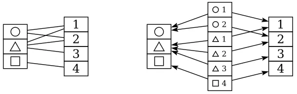
Given a set X, the functor category SetX (consideringX as a discrete category) is equivalent to the slice category Set/X. In particular, a functor of type X → Set

is an X-indexed collection of sets, whereas an object of Set/X is a set S with a functionf :S →X labelling each element ofS by some x∈X. Taking the preimage

or fiber f−1₍_x_{) of each} _x _∈ _X _{recovers an} _X_{-indexed collection of sets; conversely,}

given an X-indexed collection of sets we may take their disjoint union and construct a function assigning each element of the disjoint union its corresponding element of

X. Figure 1.1 illustrates the situation for X = {red,blue,green,purple}. Following the arrows from bottom to top, the diagram represents a functorX →Set, with each element ofX mapped to a set. Following the arrows from top to bottom, the diagram represents an object in Set/X consisting of a set of 12 elements and an assignment of a color to each.

Equivalence of categories When are two categories “the same”? In traditional category theory, founded on set theory, there are quite a few different definitions of

4_{Traditionally the notation [}

C,D] is also used, butC⇒Dis consistent with the general notation

for exponentials explained in§1.4.2; the functor category _C ⇒ D is an exponential object in the

(40)

sameness for categories. There are many different notions of “equality” (isomorphism, equivalence, . . . ), and they often do not correspond to the underlying equality on sets, so one must carefully pick and choose which notions of equality to use in which situations (and some choices might be better than others!). Many concepts come with “strict” and “weak” variants, depending on which version of equality is being used. Maintaining the principle of equivalence in this setting requires hard work and vigilence.

A na¨ıve first attempt is as follows:

Definition 1.4.1. Two categories_C and _D are isomorphic if there are inverse func-tors _C F //_D

G

o

o , such thatGF = 1_C and F G= 1_D.

This definition has the right idea in general, but it is subtly flawed. It talks about

equality of functors (GF andF Gmust beequal tothe identity). However, two functors

H and J can be isomorphic without being equal. In particular, two functors are

naturally isomorphic if there is a pair of natural transformations φ : H −→• J and

ψ : J −→• H such that φ ◦ ψ and ψ ◦ φ are both equal to the identity natural transformation. For example, consider the functors given by the Haskell types

dataRosea =Nodea [Rosea]

dataForka =Leaf a |Fork(Fork a) (Fork a)

These are obviously not equal, but they are isomorphic (though not obviously so!), in the sense that there are natural transformations,i.e.polymorphic functions,rose2fork::

∀a.Rose a → Fork a and fork2rose :: ∀a.Fork a → Rose a, such that rose2fork ◦

fork2rose =id andfork2rose◦rose2fork =id [Yorgey, 2010, Hinze and James, 2010].

Definition 1.4.1 therefore violates the principle of equivalence—to be discussed in more detail in §2.1—which states that properties of mathematical structures should be invariant under isomorphism. Here, then, is a better definition:

Definition 1.4.2. Categories_Cand_Dareequivalent if there are functors _C F //_D

G

o

which are inverse up to natural isomorphism, that is, there are natural isomorphisms 1_C∼=GF and F G∼= 1_D.

That is, the compositions of the functors F and Gdo notliterally have to be the identity functor, but only (naturally) isomorphic to it.5 This does turn out to be a well-behaved notion of sameness for categories [nLab, 2014c].

5_{The astute reader may note that the stated definition of natural isomorphism of functors}

men-tionsequality of natural isomorphism—do we also need to replace this with some sort of isomorphism

to avoid violating the principle of equivalence? Is it turtles all the way down (up)? This is a subtle point, but it turns out that there’s nothing wrong with equality of natural transformations. For the

usual notion of category, there is no higher structure after natural transformations,i.e.no nontrivial

(41)

There is much more to say about equivalence of categories;§2.1 picks up the thread with a much fuller discussion of the relationships among equivalence of categories, equality, the axiom of choice, and classical versus constructive logic.

Adjunctions The topic of adjunctions is much too large to adequately cover here. For the purposes of this dissertation, the most important form of the definition to keep in mind is that a functor F : _C → _D is left adjoint to G : _D → _C, notated

F aG, if and only if

∀AB.(F A⇒_DB)∼= (A⇒_CGB),

that is, if there is some natural isomorphism matching morphisms F A → B in the category _D with morphisms A → GB in _C. If F is left adjoint to G, we also say, symmetrically, that Gis right adjoint toF.

One example familiar to functional programmers is currying, (A×B ⇒ C)∼= (A⇒ (B ⇒ C)),

which corresponds to the adjunction

(− ×B)a(B ⇒ −).

1.4.2 Monoidal categories

Recall that a monoid is a setS equipped with an associative binary operation

:S×S →S

and a distinguished elementε :S which is an identity for. (See, for example, Yorgey [2012] for a discussion of monoids in the context of Haskell.) A monoidal category

is the appropriate “categorification” of the concept of a monoid, i.e. with the set S

replaced by a category, the binary operation by a bifunctor, and the equational laws by natural isomorphisms.

Definition 1.4.3. Formally, a monoidal category is a category _Cequipped with

• a bifunctor ⊗:_C×_C→_C;

• a distinguished object I ∈_C;

• a natural isomorphism α:∀ABC.(A⊗B)⊗C ∼=A⊗(B ⊗C); and

• natural isomorphisms λ:∀A. I⊗A∼=A and ρ:∀A. A⊗I ∼=A.

Combinatorial Species and Labelled Structures

University of Pennsylvania

ScholarlyCommons

Combinatorial Species and Labelled Structures

Brent Yorgey

Combinatorial Species and Labelled Structures

COMBINATORIAL SPECIES AND

LABELLED STRUCTURES

Brent Abraham Yorgey

A DISSERTATION

in

Computer and Information Science

Presented to the Faculties of the University of Pennsylvania

in

Partial Fulfillment of the Requirements for the

Degree of Doctor of Philosophy

2014

ὅς ἐστιν εἰκὼν τοῦ θεοῦ τοῦ ἀοράτου,

πρωτότοκος πάσης κτίσεως,

ὅτι ἐν αὐτῷ ἐκτίσθη τὰ πάντα ἐν τοῖς οὐρανοῖς

καὶ ἐπὶ τῆς γῆς, τὰ ὁρατὰ καὶ τὰ ἀόρατα,

εἴτε θρόνοι εἴτε κυριότητες εἴτε ἀρχαὶ εἴτε

ἐξουσίαι· τὰ πάντα δι’ αὐτοῦ καὶ εἰς αὐτὸν

ἔκτισται·

καὶ αὐτός ἐστιν πρὸ πάντων

καὶ τὰ πάντα ἐν αὐτῷ συνέστηκεν,

καὶ αὐτός ἐστιν ἡ κεφαλὴ τοῦ σώματος τῆς

ἐκ-κλησίας·

ὅς ἐστιν ἀρχή,

πρωτότοκος ἐκ τῶν νεκρῶν, ἵνα γένηται ἐν πᾶσιν

αὐτὸς πρωτεύων,

ὅτι ἐν αὐτῷ εὐδόκησεν πᾶν τὸ πλήρωμα κατοικῆσαι

καὶ δι’ αὐτοῦ ἀποκαταλλάξαι τὰ πάντα εἰς

αὐτόν, εἰρηνοποιήσας διὰ τοῦ αἵματος τοῦ

σταυροῦ αὐτοῦ, εἴτε τὰ ἐπὶ τῆς γῆς εἴτε τὰ

ἐν τοῖς οὐρανοῖς·

Acknowledgments

Statement of contribution

ABSTRACT

Contents

List of Tables

List of Figures

Chapter 0

Introduction

Chapter 1

Preliminaries

1.1

Metavariable conventions and notation

1.2

Set theory

1.3

Homotopy type theory

1.3.1

Terms and types

1.3.2

Equality

1.3.3

Path induction

1.3.4

Equivalence and univalence

1.3.5

Propositions, sets, and

n

-types

1.3.6

Higher inductive types

1.3.7

Truncation

1.3.8

Why HoTT?

1.4

Category theory

1.4.1

Category theory fundamentals

J

K

E

L

I

B