PATTERNS FORMATION IN A PMZC PLANKTON MODEL
Tahani Al-Karkhi
Department of Mathematical Sciences, University of Essex, UK
Wivenhoe Park, Colchester, CO4 3SQ, United Kingdom
Abstract
In this paper, we focus on the phenomenon of pattern formation in a reaction diffusion model of plankton dynamics, which includes support for infochemically mediated trophic interactions. We consider a four species model created on the basis of the two species models which have been studied previously. In our model, which is an extended version of these previous models, the grazing pressure of microzooplankton (M) on phytoplankton (P) is controlled through external infochemically (C) mediated predation by copepods (Z). We undertake a stability analysis of both the two species and the four species models and compare their system dynamics. We compared the mathematical roots related to these models using both numerical and analytical methods, and we found consistency between the two approaches using asymptotic expansion. We also explored spatial pattern formation in relation to both forms of model and considered under what conditions Turing patterns are exhibited and when spatiotemporal chaos can be observed. An attempt was made to study the non-Turing patterns, which were discovered with a special emphasis on spatiotemporal chaos.
Keywords:
Plankton model, Plankton dynamics, Infochemicals, PMZC-model, Asymptotic Expansion Analysis, Limit cycle, Dynamical system, Chaos, Systematic analysis, Food-webs, Multitrophic interactions.
1. Introduction
190202-4848- IJBAS-IJENS @ April 2019 IJENS I J E N S indicate the interaction directions. There are four interacting components, namely the phytoplankton (P), the microzooplankton (M), the zooplankton (Z), and the infochemical release, (C) as shown in Fig.(1). The interactions shown in the diagram are described by a system of four differential equations, below is a full description of the PMZC-model.
Where U represents a vector of four components: P denotes the population density of the prey phytoplankton, M denotes the population density of the predator microzooplankton, and Z denotes the population density of the top predator (copepods), all at time T; i = 1,2,3,4 indicates the num-
Figure 1: Schematic diagram of proposed model
ber of species in the community, C denotes the effect of prey (copepods) on trophic interactions, and functions Fi take into account the effects of birth and mortality. In most biologically meaningful situations, the functions Fi are nonlinear with
respect to at least some of their arguments. In the second part of the above equation, D∇2U indicates that the simplest
(2)
Keeping in view the above discussion, we study a plankton model supporting a one prey and two-predator system with Holling type II functional responses Fig.1. The main contribution of this paper is to expand the two trophic model studied by (Lewis et al., 2012) to a four trophic model and then study the effect of diffusion on the resultant four species food web model (which retains the Holling type II functional responses).
190202-4848- IJBAS-IJENS @ April 2019 IJENS I J E N S studies in the ecological field pay particular attention to the practical contexts of spatial processes (Baurmann et al., 2004). The remainder of this paper is organized as follows: in Section 2, we propose the spatiotemporal PMZC model; Section 3 presents an asymptotic expansion analysis; this is followed by Section 4 which presents a local stability analysis and indicates the limit cycle condition for the temporal system; In Section 5, we derive the analytical conditions for diffusion driven instability using the Ruth Hurwitz criteria. Also in that section we provide the results of the numerical simulation, which was performed; in Section 6, the systematic analysis is discussed; and finally, conclusions are given in the last section, Section 7.
2. The temporal PMZC-Model
A mathematical model was developed of the situation whereby one prey species is utilized by two predator species and this model included the chemical releases involved; this was studied within a temporal domain and with Holling type II functional responses (Holling, 1965). Motivated by the work (Lewis et al., 2012), we derived Fi, i = 1..4, which is the interaction function for the model which we have developed. The interaction function has the following format:
,
(3)
(4)
(5)
(6)
(7)
,(8)
(9)
(10)
The above model describes the interactions between the small infochemical producing phytoplankton, the microzooplankton and the copepods in a system that is depleted of nutrients. The parameter, r, represents the phytoplankton intrinsic growth rate, a is the clearance rate of microzooplankton at low food densities, bi i = 1,2 represents the half saturation constants, β is the copepod linear predation rate, mi (i = 1,2) are the predators death rates, m3 is the chemical evaporation rate,
and is a key parameter that we use to reduce the general four species model to a special case model, i.e., that of (Lewis et al., 2012). η is the productivity rate of the DMS-infochemicals, and ω is the amount of chemical given off by each phytoplankton.
In Eq. (7), we employ a logistic map to describe the growth rate of prey and a Holling II functional response to describe the effects predators have on (the microzooplankton) prey. In Eq. (8), we define the microzooplankton population growth using a Holling II functional response with γ1 as a conversion parameter — this latter regulates the conversion of prey biomass into
predator biomass. The second term in Eq.(8) represents the normal (non-predator-induced) mortality of microzooplankton, while the third term represents the effects of zooplankton on microzooplankton— of course, zooplankton provides another source of microzooplankton mortality. The third term represents the increase in predation with β as a linear predation rate 1.
Copepods saturate w.r.t. their predation activities according to their behaviour when handling their prey (microzooplankton), with b2 being the half saturation parameter. The chemicals released could also be saturated via the (1 + C) factor, and the ζ
parameter is used to measure the rate of chemical increase (that effects increases in predation 2. In Eq. (9) the first term we
introduce is the copepod population growth which connects both predator populations, M and Z. This term also describes how copepods consume microzooplankton following DMS release and how copepods saturate because of the time it takes to handle prey. The next term represents copepod mortality due to their consumption by higher trophic predation. The final equation (10) has three terms. The first term is used to describe the infochemical release following the start of microzooplankton grazing on phytoplankton; η is the productivity rate of DMS. The second term in F4 stands for chemical evaporation. The third term
represents the level of chemical (exudation) release by each cell. We can reduce the model in Eqs. (7)- (10) into a special case
model by setting = 0, i.e:
The main difference between the two set of nonlinearities and the model represented by Eq. (14) is the linear predation function, which describes the linear effects of the predation by copepods of microzooplankton. It can be assumed that the
1 -β MZ represents the effects of the copepods on the microzooplankton; any species should saturate at some level.
Therefore we changed the layout of this term to that of a Holling II functional response.
2 also can be defined as the maximum level of chemical, which can be released, especially if we model this
190202-4848- IJBAS-IJENS @ April 2019 IJENS I J E N S model is valid over significant periods of time–scales because we have included resources which are in addition to the basic food chain of the two species model: i.e., the infochemical releases (by the phytoprotozoa) and the population density of the copepods. Thus, we must consider the time that both predators M and Z take to handle their prey. The model represented by
Eq. (14) is considered as a special case of the models represent by Eqs. (7) - (10). This is because, when = 0 the model is reduced to the two species model as in (Lewis et al., 2012). One goal of the model construction undertaken here is to predict the predator–prey kinetic and dynamic properties. Since our model is constructed from the two species predator– prey model P and M, a basic question to raise here is how can the four species model provide for more descriptive power than the two species model?
3. Qualitative analysis of the location of the equilibria
Here we look for the steady-state solutions (P,M,Z,C) which satisfy ) = 0. The system shown in Eqs. (7)-(10) possesses five possible nonnegative equilibria: namely, the extinction equilibrium E0; the microzooplankton and
copepod-eradication equilibrium E1; the phytoplankton and infochemical eradication equilibrium E2; the copepod (free)
eradication equilibrium E3; and finally the coexistence equilibrium E4. Table 3 shows the number of equilibria and their types
and definitions.
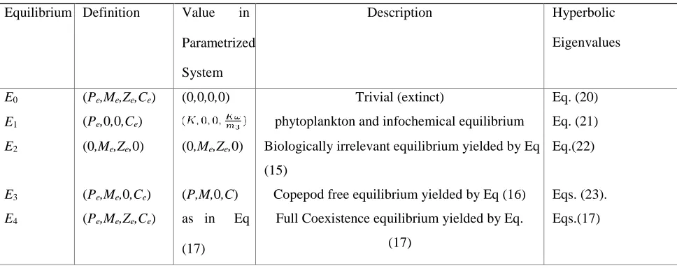
Table 1: All possible equilibria of the system given by Eqs. (7)-(10) both biologically relevant and irrelevant. Equilibrium Definition Value in
Parametrized
System
Description Hyperbolic
Eigenvalues
E0 (Pe,Me,Ze,Ce) (0,0,0,0) Trivial (extinct) Eq. (20)
E1 (Pe,0,0,Ce) phytoplankton and infochemical equilibrium Eq. (21)
E2 (0,Me,Ze,0) (0,Me,Ze,0) Biologically irrelevant equilibrium yielded by Eq
(15)
Eq.(22)
E3 (Pe,Me,0,Ce) (P,M,0,C) Copepod free equilibrium yielded by Eq (16) Eqs. (23).
E4 (Pe,Me,Ze,Ce) as in Eq
(17)
Full Coexistence equilibrium yielded by Eq. (17)
Eqs.(17)
The biologically irrelevant equilibrium is yielded by:
. (15)
. (16)
The full co-existence state satisfies the quartic polynomial
Where Ai, i = 0,..,4 are cascading parameters as given in Appendix A. While M, Z and C are given by
,
Z(Pe) = A5(Pe)2 + B(Pe) + G, (18)
.
The persistent full co-existence is state yielded by a quartic polynomial as follows;
(19)
Where Ai, i = 0,..,4 are all cascading parameters (provided in Appendix C).
3.1. System behaviour near the origin E0
A straightforward calculation shows that the hyperbolic equilibrium, which is the first trivial (extinction) equilibrium, is an unstable saddle point, with the unstable manifold in the direction orthogonal to the M−Z−C coordinate
plane.
λE0 = (r,−m1,−m2,−m3) (20)
3.2. System behaviour near the microzooplankton and copepod eradication equilibrium E1
The E1 equilibrium point of the system, which entails microzooplankton and copepod eradication, is locally
190202-4848- IJBAS-IJENS @ April 2019 IJENS I J E N S stable. The eigenvalues of the second microzooplankton and copepod eradication equilibrium are:
3.3. System behaviour near the phytoplankton and infochemical eradication equilibrium E2
The Jacobian matrix of the system 10 around the, non-feasible, phytoplankton and infochemical eradication equilibrium point, E2, yields the following eigenvalues.
Where all its coefficients are given in Appendix 3 Now, this hyperbolic point is an unstable saddle, since all the parameters are positive: λ1 is unstable; also, because λ2,3 have negative real parts, these are stable foci. Further, since λ4 < 0 we have a
saddle-focus point, as when we have one real eigenvalue with the opposite sign to that of the real part of a pair of complex-conjugate eigenvalues and a negative real fourth eigenvalue; This type of equilibrium is always unstable.
3.4. System behaviour near the copepod eradication equilibrium E3
The Jacobian matrix of the system 10 for the fourth equilibrium (with copepod eradication) has the following four eigenvalues:
(23)
Where A and B are as in Appendix 2. This hyperbolic point is unstable since all the parameters are positive. And λ1 is
unstable if A > B > 0, and because λ2,3 have negative real parts, these are stable foci, and since λ4 < 0, we have a saddle-focus
point — as when we have one real eigenvalue with the opposite sign to that of the real part of a pair of complex-conjugate eigenvalues and a negative real fourth eigenvalue; This type of equilibrium is always unstable.
3.5. System behaviour around the coexistence equilibrium point E4
The relevant Jacobian matrix is J4 = (aij)4×4. Let λi, i = 1,2,3,4 be the roots of the characteristic polynomial of J4 which is
given by:
Where Ai are cascading parameters given in Appendix D and A0 = 1. From the Routh-Hurwitz criterion, all the roots of a
Jacobian matrix have negative real part if and only if the determinants of all the Harwitz matrices are positive (Porter, 1968), and then any E is locally asymptotically stable if and only if A1 > 0, A3 > 0 and A1A2 > A3 and A3 > pA1(A1A4 − A2A3) or
.
Obviously, we have A1 < 0 and A3 < 0 and by depending on the Jacobian element matrix, when a12 < 0, a21 > 0, a23 < 0, a32 >
0, a33 < 0 and a44 < 0. It is readily seen that A1A2A3 > . Therefore, we formulate the necessary and sufficient
conditions for the positive equilibrium to be locally asymptotically stable; these follows from the Routh Hurwitz criterion. For this purpose, we use the notation given in appendix.
4. Asymptotic Expansion Analysis
Using an asymptotic approach it is possible to make some limited analytical progress with the general system given in Eqs.(10). In this analysis, we study how to scale our parameters in order to determine the general stability for PMZC-models’ roots. We can start performing the method by setting the following assumption:
,
. and by substitute our scaled parameters
and the following expansion into the full co-existence persistence state, which is given by 17:
(25)
we will obtain an expanded polynomial, by collecting the coefficient of its leading order we could obtain the appropriate value of prey density Pe. Which
is:
(26)
190202-4848- IJBAS-IJENS @ April 2019 IJENS I J E N S Now, after determine the values of scaled root E4, we could study the general stability analysis by following the same
procedures method we presented on this section i.e
(27)
An expanded characteristic polynomial could be obtained following the same procedures and by substituting 27 and collecting the coefficient of the leading order and then solve for λ, we could obtain the following eigenvalues:
. (28)
and by substituting the analytically derived value of P into the quadratic polynomials of M and C and the fractional polynomial of Z we obtain:
After determining the values of the scaled root, E4, we can undertake a general stability analysis by following the same
procedures. After determining the characteristic polynomial of the model in Eq. 6 from the Jacobian matrix, we expand λ as
in Eq. 29and substitute it back into the characteristic polynomial.
(29)
and by collecting the coefficient of the leading order, we will determine four eigenvalues as follows:
Figure 2: A comparison between the numerical and the analytical approaches used to solve the quantic polynomial of the four species model in Eq.6.
Where A, B, α and β are all cascading parameters: the formula is quite prolix, so it has been moved to the appendix. Comparing the analytical roots and eigenvalues of the system, 6, with the numerical results shows that all the results are consistent. Fig. 2 illustrates the consistency of the two approaches.
5. Parameter Values Investigation
A major reason for modelling the dynamics of a population is to understand its principle controlling features and so be able to predict the likely pattern of development consequent upon a change of environmental parameters (Murray, 2002). In the PMZC model of 10 we assumed that the parameters within the elementary analysis are similar to their values as given previously (Lewis et al., 2012).We denote these values as default values. It was apparent that oscillatory solutions were present in the two models, when κ = b2 = ω = 0 and when κ = 1, b2 = 0.05, ω = 0.1; this makes the two sys-
tems presented here consistent with the results which were found previously:
i.e. the model relaxes to a stable steady state. However, in this paper we are concerned with a 4 species system. Therefore, we need to consider carefully the effects of each parameter on the PMZC food chain; this might help us to obtain a valid solution (model) especially with respect to the fact that we are introducing the effects of zooplankton into this system. Following (Edwards and Brindley, 1999), the parameter values used to model the zooplankton mortality can have a major influence on the dynamics of simple models (Edwards and Yool, 2000), (Edwards and Brindley, 1999). They found that, for their particular parameter values, the limit cycle behaviours (unforced oscillations) which occurred when they used a linear zooplankton mortality term did not occur when they used a quadratic term. With respect to (Lewis et al., 2012) and (Morozov et al., 2010), we keep the maximum growth rate parameter of these logistic growth models in the range 0.1 < r < 2d−1. In (Franks, 2001), the phytoplankton carrying capacity was set to K = 50µgCI−1, but (Morozov et al., 2010) considered a much wider range K = ∞. Therefore, we use 50 < K < ∞ (Edwards and Brindley, 1999).
(Edwards and Brindley, 1999), (Saiz and Calbet, 2007) estimated the half saturation constant of phytoplankton to be in the range 20 < b1 <
150µgCI−1, and the zooplankton (copepod) half saturation constant to be 20 < b2 < 100µgCI−1 — to reflect the fact that
copepod dynamics develop on a slower time scale than microzooplankton dynamics. However, because we are introducing zooplankton (copepods) and we are going to study their effects on the food chain, the more accurate values for b1 and b2 which
will be used in this model is much smaller than the literature suggests. We will set a very small value for the zooplankton (copepod) population density, in contrast to that set for microzooplankton. This is because we are not introducing any higher trophic, and because the model is non-nutrient limited in particular circumstances. We have chosen the b1P and b2M terms in
the way that we have because these terms may be regarded as reflecting the amount of time it takes for the predators to handle
their prey (Cantrell and Cosner, 2004), and if we choose 0, then the predator density will tend to zero over time.
190202-4848- IJBAS-IJENS @ April 2019 IJENS I J E N S . In this model, we cannot choose b2 > b1 for the same reasons.
In (Strom and Morello, 1998), the microzooplankton conversion efficiency is estimated to be 0.15 < γ1 < 0.64, but
(Kiørboe, 2008) states that the conversion efficiency may be higher when considering zooplankton feeding on microplankton; hence, here, a higher value of γ2 = 0.7 is chosen for the copepod assimilation efficiency. Also, the maximum copepod predation
rate was chosen to be β = 1d−1. In our model, copepods are specified as having a default mortality value; we didn’t take into
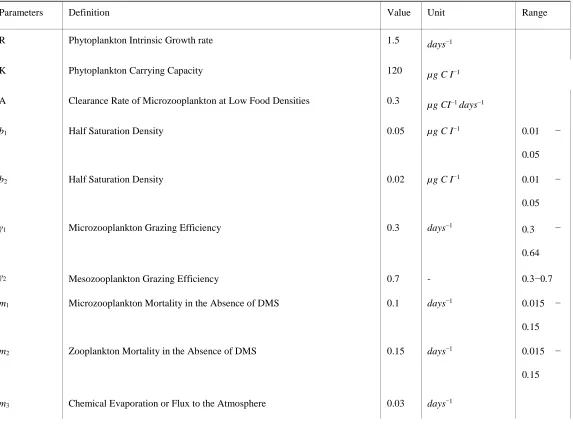
Table 2: Outline descriptions, default values and the ranges of the parameters: the ranges presented cover values used by a variety of authors for different models.(Edwards and Brindley, 1999), (Edwards and Yool, 2000) and (Saiz and Calbet, 2007).
Parameters Definition Value Unit Range
R Phytoplankton Intrinsic Growth rate 1.5 days−1
K Phytoplankton Carrying Capacity 120 µg C I−1
A Clearance Rate of Microzooplankton at Low Food Densities 0.3 µg CI−1 days−1
b1 Half Saturation Density 0.05 µg C I−1 0.01
0.05 −
b2 Half Saturation Density 0.02 µg C I−1 0.01
0.05 −
γ1 Microzooplankton Grazing Efficiency 0.3 days−1 0.3
0.64 −
γ2 Mesozooplankton Grazing Efficiency 0.7 - 0.3−0.7
m1 Microzooplankton Mortality in the Absence of DMS 0.1 days−1 0.015
0.15 −
m2 Zooplankton Mortality in the Absence of DMS 0.15 days−1 0.015
0.15 −
η DMS Production Rate 0.1 -
β Mesozooplankton Linear Predation Term 1 -
ζ Chemical Release, Rate of Increase CP -
6. Mathematical analysis and results
6.1. Time Series and Phase Portraits
The main objective of this section is to support the analytical findings with the help of experimental parameter values derived from the published literature — as presented in table 2. This table is of the 14 parameters used in the model 10 across the same range as the range of the parameters shown in my previous work on two species spatial analysis. Also the values of these parameters are closely related to the value of the main control parameters, ν and m3, that helped us to set initial
condition/prediction (IC) for the numerical analysis (in order to obtain consistent results). One of the main purposes of this section is to verify our analytical findings (in Table 3) using numerical methods. The numerical simulations illustrate a number of important features of the system from a practical point of view. Figure 3 exhibits the local stability of the model around a proposed initial condition; we set this condition in order to test the consistency between the two species model and the expanded model (with the parameter values given in table 2).
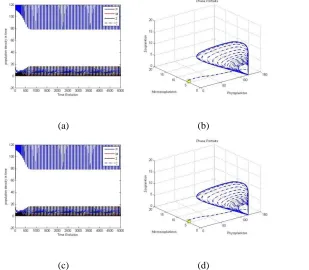
In figure 3, the development over time plot is of the special case model and the trajectory in PMZC space of the system from the proposed initial condition (Pe,Me,Ze,Ce) = (3.942,5.789,0.0481,20.379) and ζ = 0.01 (and all other parameters fixed at
their default values). In 3(b), it is shown that the trajectory is attracted onto a limit cycle with a specific period of roughly 500 days. The trajectory exhibits large-amplitude fluctuations in P.
The dynamics of the prey-dependent model are: stable coexistence, unstable coexistence, or extinction of the predator.
(a) (b)
(c) (d)
Figure 3: Time series and phase-space trajectories around the proposed initial condition for the two cases of PMZC system put forward here: all of the other parameters (not included in the set initial condition) are fixed as in table 2 — also ζ = 0.01. In
190202-4848- IJBAS-IJENS @ April 2019 IJENS I J E N S
(a) (b)
Figure 4: Time series and phase portraits near the microzooplankton and copepod eradication equilibrium point, E1 and ζ =
0.01.It is readily seen that the trajectories are attracted onto a stable limit cycle
(a) (b)
Figure 5: Time series and phase portraits of (copepod free) equilibrium point E3 withζ = 0.01 and all other parameters fixed as
in 2. The trajectories are attracted onto a stable limit cycle.
(a) (b)
Figure 6: Time Series and phase portraits around the coexistence equilibrium point E4 with ζ = 0.01 and all the other parameters
and in black. The limit-cycle represents the overall movement over the time series, ignoring seasonality and any small random fluctuations. In 6(b), It is illustrated that the trajectories are attracted onto a stable limit cycle.
6.2. One parameter bifurcation behaviour
We have used numerical simulations of the proposed model 10. Figure 7 represents the local stability diagram around E4
with the parameter values given in table 2. It is readily seen that 7(a) indicates that if in the coexistence equilibrium E4 < K then
the population of phytoplankton will bloom. Especially, if E4 is a function of ζ; this can be seen to reflect the consistency
between our previous work and this current study. However, if E4 > K then the prey population will decrease significantly.
Also, if E4 = K then the population will remain constant (Freedman, 1980).
These graphs illustrate the PMZC biological model. When a specific choice of parameters is made, the prey population increases to extremely high numbers in each cycle and then recovers (while the predator population remains sizeable as at the highest prey density). In real-life situations, how-
(a) (b)
(c) (d)
Figure 7: The coexistent equilibrium point w.r.t ζ as an infochemical metric, shows that the range of our control parameter should be 0 < ζ < 0.1 to avoid having negative real roots for Z.
190202-4848- IJBAS-IJENS @ April 2019 IJENS I J E N S 7. Turing Analysis in Relation to the PMZC Model
Several studies have been devoted to the various modes of spatiotemporal organization generated by different models: e.g., limit cycles, Turing patterns, and traveling waves in one-dimensional systems ().The interest in this paper is to provide a fundamental understanding of how a steady state that is locally asymptotically stable in a non-spatial system can become unstable in a corresponding diffusive system. Consider the system in 1, where Ui and i = 1,2,3,4 represent a vector of the system state variables P,M,Z,C at position X and time t. It is readily seen that, in the vicinity of a spatial homogeneous steady state (Pe,Me,Ze,Ce), the corresponding linearized system has the following form:
(30)
where Ui = P,M,Z,C, and i = 1,..,4 this is in the case of a spatially homogeneous perturbation, and
In the case of a spatially inhomogeneous perturbation with k as a wave number. Here and δij is the Kronecker symbol, and Ui(t) and Ui(t,k) are the amplitudes of the perturbation and its Fourier transform, respectively (Malchow, 1993). It is readily seen that when k = 0, the system given by 30 coincides with that in 31. The matrix of the linearised system is shown in Appendix B. We obtained the dispersion relation as a quartic polynomial and by solving this polynomial for δ we can study
the Turing
instability conditions.
, (32)
Where Pi are all cascading parameters, all the related details are given in Appendix C. It is apparent that, according to the analytical break-down shown in table 3, E1 is a steady state of the system 10, called the phytoplankton and infochemical
equilibrium. This state is stable under the common two conditions trace(A) < 0 and a11 + a22 + a33 + a44 < 0. Spatiotemporal
chaos arises from the diffusive coupling of local limit cycle oscillators (Malchow et al., 2008); the patterns so generated in two- and three-dimensional systems include patterns arising from the interference of different instability mechanisms.
8. Spatial Distribution and Limit Cycles
In this section we consider the model in Eq. (1) as it exists in continuous time and space. The model is of four interacting species and represents an example of a community population with an oscillatory solution. Here we are interested in the possible emergence of non-Turing, Turing, and limit cycle patterns. First, we assume that the diffusivity is the same for all species, and then we assume that DC < DM < DZ < DP . However, it appears that the choice of initial condition, as given in Eq. (33), could affect the types of pattern which is generated (Murray, 2002). Fig’s 8 and 9 show the one dimensional systematic analysis of Eq. (1), starting from the types of the patterns and the behaviour of the system in time and space. The PMZC model can generate
a number of quite different patterns, depending on the choice of initial condition.
. (33)
The type of system dynamics exhibited depends significantly on the choice of the initial conditions (Malchow et al., 2008).
190202-4848- IJBAS-IJENS @ April 2019 IJENS I J E N S condition is imposed. Non-Turing patterns result when we perturb the initial distribution by adding terms like and δ into the two dimensional initial distribution below:,
(34)
Where the values for the important terms, and δ in Eqs. (34) are given as follows:
(a)
(b)
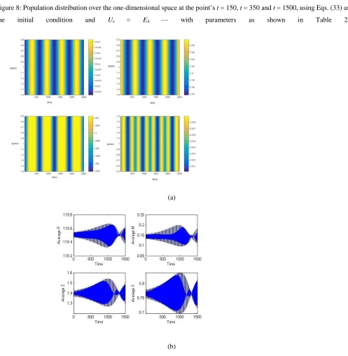
190202-4848- IJBAS-IJENS @ April 2019 IJENS I J E N S Figure 8: Population distribution over the one-dimensional space at the point’s t = 150, t = 350 and t = 1500, using Eqs. (33) as the initial condition and Ue = E4 — with parameters as shown in Table 2.
(a)
(b)
Figure 9: Schematic analysis, with respect to space and time, of Eqs. (10) and of the average density of PMZC in time, using Eqs. (33) as the initial condition and Ue = E4.
Figures 8(a), 8(b) and 8(c) show the population densities generated by the dynamics variables at times t = 150, 350 and 1500, using Ue = E4. Fig. 8(c) shows the regularity of the oscillatory solution of the population densities given by the dynamics
(a)
(b)
(c)
190202-4848- IJBAS-IJENS @ April 2019 IJENS I J E N S (a)
(b)
(c)
Figure 11: The population distribution over the one dimensional space at the point t = 1500 plus the correspondent schematics analysis across space and time, Eqs. (10); also the average density of PMZC over time, using Eqs. (33) as the initial condition, E1, for ζ = 0.001; other parameters are as in 2.
(a) (b)
(c) (d)
(e) (f)
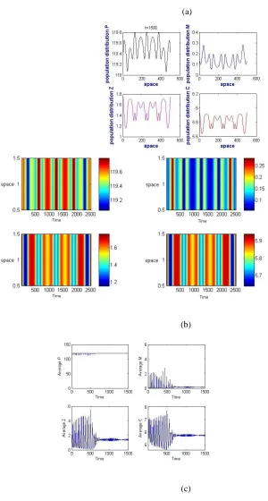
Figure 12: Non-Turing patterns in a predator-prey distribution over the two dimensional space relating to the times t = 150, t = 180 and t = 1500, using Eq. (33) as the initial condition and Ue = E4, with parameters as shown in Table 2. In Fig .12, the spatial
distributions of a prey species at different times is presented in order to show the continuous changes in the distribution of species. Patterns are presented here which were generated within the time span t = 10 to t = 1500, but the existence of similar patterns was verified for longer duration simulations. This type of pattern is classified as a stripes patterns and is a non-Turing pattern because not all the Turing conditions hold. In Fig. 13, we find another non-Turing pattern, generated by the PMZC model when ζ = 0.001 and when a suitable choice of the parameters such that DC < DM < DZ < DP was made; this analysis was
190202-4848- IJBAS-IJENS @ April 2019 IJENS I J E N S concentrations of both prey and predators. The non-Turing patterns observed for the classical Holling-functional response are of two types: hot spot patterns and cold spot patterns. Hot spots consist of localized circular patches with high population densities. Our stationary cold spot pattern changed to a chaos pattern due to the coalescence of nearby circular patches with low population densities. The stationary patterns obtained for the PMZC model are completely independent of the initial condition. We have checked this independence numerically, by using E4 as an initial guess, without perturbing it, we obtained
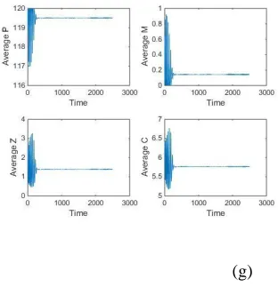
a flat state. This unstable steady-state property of the non-stationary patterns is illustrated in Fig.12 and 13, where the spatial averages of the population densities are plotted against the space dimension, as in 12(e), and against the time dimension, as in 12(f). It is
(a) (b)
(c) (d)
(g)
Figure 13: Non-Turing patterns for predator-prey distribution over a two dimensional space representing prey and predator for t = 150,350 and t = 1500, using Eq.34 as I.C. with Ue = E4 and ζ = 0.001; all other parameters are as shown in Table 2.
Important to note here that the temporal steady state is unstable and oscillates for ζ ≥ 0.001. Further analysis is performed in
order to investigate other biologically relevant equilibria which were generated in order to obtain some specific patterns; the patterns yielded vary according to the choice of the initial condition and the type of the equilibrium. See Fig. (14).
The patterns produced by the PMZC model 1 can be in the form of a stripe-like arrangement of activated cells (in terms of phytoplankton concentrations)3; alternatively, active spots can lead to chaos. E
1,E3 and E4 are unstable equilibriums of the
non-spatial model: Eqs.7–, 10, ⇒<(λ) > 0. The Turing conditions are not satisfied and this gives rise to chaos patterns in the spatial
system because ⇒ λ(k2) > 0. Spatiotemporal chaos arises from a diffusive coupling system of equations with local limit cycle
oscillators(Malchow et al., 2008); spatiotemporal patterns depend on the choice of the initial conditions. Infochemically mediated interactions can have a strong effect on the structuring, functioning and composition of marine ecosystems. For example, it has been observed that chemical gradients play a key role in generating complex patterns and in cell differentiation (Steinke et al., 2006).
190202-4848- IJBAS-IJENS @ April 2019 IJENS I J E N S
(a) (b)
(c) (d)
(e)
Figure 14: Non-Turing patterns generated by Eq. (1), using the initial conditions from Eq. (34) with Ue = E1 and ζ = 0.001; other
190202-4848- IJBAS-IJENS @ April 2019 IJENS I J E N S
(a) (b)
(c) (d)
Figure 15: Non-Turing patterns generated by Eq. (1), using the initial conditions from Eq. (34) with Ue = E3 and ζ = 0.001;
190202-4848- IJBAS-IJENS @ April 2019 IJENS I J E N S Table 3: Spatial Analysis of the four species model presented in Eq. (1).
Equilibrium Description Turing Conditions Routh–Hurwitz Criterion
Type of pat-
terns
E0 Trivial (eradication) λ(k2) >
0 and
H(k2)
P1 > 0,
E1 Phytoplankton and
infochemical equilibrium
λ(k2) >
0 and
H(k2) <
0
P1 > 0, Stripes patterns using
Eq.33 as I.C. and spots
pattern using Eq.34 as I.C.
E2 Biologically irrelevant
equilibrium as given in Eq. (15)
λ(k2) >
0 and
H(k2) >
0
P1 > 0, Stripes patterns using
Eq.33 as I.C. and spots
pattern using Eq.34 as I.C.
E3 Copepod eradication
equilibrium given by Eq. (16)
λ(k2) >
0 and
H(k2) >
0
P1 > 0, Stripes patterns using
Eq.33 as I.C. and spots
pattern using Eq.34 as I.C.
E4 Full Coexistence
equilibrium given by Eq. (17)
λ(k2) >
0 and
H(k2) >
0
P1 > 0, Stripes patterns using
Eq.33 as I.C. and spots
190202-4848- IJBAS-IJENS @ April 2019 IJENS I J E N S 9. Acknowledgment
Tahani Al-Karkhi gratefully acknowledges financial support from the Ministry of Higher Education and Scientific Research in Iraq/Baghdad for the fund provided to implement this work. Also, she is grateful to her supervisors Hadi Susanto and Edward Codling for their help and support provided to improve the PMZC model and perform the results in a presentable way.
10. Conclusion
In this paper, a one prey and two predator system with Holling type II functional responses has been considered. It is shown that there exists a limit cycle with respect to the chemical release, ζ, in relation to the spatially homogeneous system as given
in fig.7. In the qualitative analysis of Eq. 1, we studied the dynamical behaviour of the temporal system. It was established that when the rate of mutual interference of the predator (i.e., M and Z), crosses a threshold value (i.e., M = M0 and Z = Z0) then
prey, first predator and second predator populations start oscillating around the interior equilibrium as shown in Fig.7. The dynamics of spatially inhomogeneous aquatic communities has been illustrated in this chapter by studying Turing instability in the PMZC model, using the Routh Hurwitz criteria (DeJesus and Kaufman, 1987). The Turing criteria did not hold in relation to this study because, as we have remarked earlier, the coexistence point, E4, possesses four eigenvalues and two of these
represent an unstable focus (with Re(λ) > 0) and the other two stable sinks. Furthermore, based on the numerical experiments,
190202-4848- IJBAS-IJENS @ April 2019 IJENS I J E N S Banerjee, 2012)). Also, we could provide a more detailed explanation of the sort of patterns that were yielded by studying further the dispersion relation of the model as it is when we obtain the striped patterns given in Fig. 12, because we used a periodic function as an initial condition for Eq. (33). As found in (Genieys et al., 2006), we can expect the existence of oscillatory travelling waves and more complex, for instance modulated, spatio–temporal dynamics. Spatiotemporal patterns exists for the parameter values given in Table 2. In Fig 13, using the parameter values shown in Table 2 but different initial conditions such as the initial conditions given in Eq. (34), we observed a pattern formation with a number of different time steps. Also, it can be observed that the stationary ”mixtures −→ stripe–spot mixtures −→ spots” patterns are time-dependent, as was found in (Malchow et al., 2008). These observations confirm the fact that the interactions between the temporal and the spatial aspects are unable to drive the system towards spatial and temporal irregularity under any circumstances. The existence of irregular distributions of populations over space and continuous changes to these over time depends on complex interactions which take place over both the spatial and temporal scales. Finally, all these spatial patterns show that qualitative changes lead to different spatial density distributions for each species, across the spatial system. Furthermore, we analysed the stability of the linear and non-linear systems with the help of a Turing instability analysis and observed that the spatiotemporal system in Eq. (1) does not change its behaviour: as revealed by the spatial systematic analyses shown in Figs. 8 and 9 for one dimension; and Figs. 12, 12(e), 12(f), 13 and 13(g) for two dimensions. This is because the trajectories are spiralling in a limit cycle and thus they tend to converge into a stable point. Our results show that modeling by reaction –diffusion equation is an appropriate way to investigate the fundamental mechanisms of the spatio-temporal dynamics of the real world food web system (Petrovskii and Malchow, 1999) and (Baghel et al., 2014).
11. Appendix
A. The cascading parameters of the coexistence point
A0 = γ2b1βηr2 + ζb1βηr2 − b1b2ηm2r2,
A1 = −2γ2b1βηkr2 − 2ζb1βηkr2 + 2b1b2ηkm2r2 − γ2b1βkωr − ζb1βkωr
+ b1b2km2ωr + γ2βηr2 + ζβηr2 − b2ηm2r2,
A2 = −γ2b1βηk2r2 + ζb1βηk2r2 − b1b2ηk2m2r2 + γ2b1βk2ωr
190202-4848- IJBAS-IJENS @ April 2019 IJENS I J E N S + b1b2km2m3r + 2b2ηkm2r − γ2βkωr − ζβkωr + aηkm2r + b2km2ωr,
A3 = γ2b1βk2rm3 + γ2βηk2r2 + ζβηk2r2 − b1b2k2rm2m3
− b2ηk2r2m2 + γ2βk2ωr + ζβk2ωr − aηk2rm2 − b2k2ωrm2
− γ2βkrm3 − ak2ωm2 + b2krm2m3,
A4 = γ2βk2m3r − b2k2m2m3r − ak2m2m3,
B. The details of the fourth eigenvalue correspond to E2
A0 = γ1ak(γ1a − b1m1) (B.1)
+ γ12a2b21k2m21r2 + 4γ1ab13k2m14r − 2γ1ab31k2m31r2
+ b41k2m41r2 + 4γ13a3km21r − 8γ12a2b1km31r
− 2γ12a2b1km21r2 + 4γ1ab21km14r + 2b31km41r2
+ γ12a2m21r2 + 2γ1ab1m31r2
190202-4848- IJBAS-IJENS @ April 2019 IJENS I J E N S C. The cascading value of A and B of the eigenvalue correspond to the equilibria E3.
A = −γ14γ2a3βk2m3r + γ14a3b2k2m2m3r + 3γ13γ2a2b1βk2m1m3r
− γ13γ2a2βηk2m1r2 − γ13ζa2βηk2m1r2
− 3γ13a2b1b2k2m1m2m3r + γ13a2b2ηk2m1m2r2 − 3γ12γ2ab12βk2m21m3r
+ 2γ12γ2ab1βηk2m21r2 + 2γ12ζab1βηk2m21r2
+ 3γ12ab21b2k2m21m2m3r − 2γ12ab1b2ηk2m21m2r2 + γ1γ2b31βk2m31m3r
+ γ1γ2b21βηk2m31r2 − γ1ζb21βηk2m13r2 + γ1b31b2k2m31m2m3r
+ γ1b21b2ηk2m31m2r2 + γ14a4k2m2m3 − γ13γ2a2βk2m1ωr
− γ13ζa2βk2m1ωr + 4γ13a3b1k2m1m2m3 − γ13a3ηk2m1m2r + γ13a2b2k2m1m2ωr − 2γ12γ2ab1βk2m12ωr − 2γ12ζab1βk2m21ωr
+ 6γ12a2b21k2m21m2m3 + 3γ12a2b1ηk2m21m2r + 2γ12ab1b2k2m12m2ωr
− γ1γ2b21βk2m31ωr + γ1ζb21βk2m31ωr + 4γ1ab31k2m31m2m3
+ 3γ1ab21ηk2m31m2r − γ1b21b2k2m13m2ωr − b41k2m41m2m3
− b31ηk2m41m2r − γ13γ2a2βkm1m3r − γ13a3k2m1m2ω
− γ13a2b2km1m2m3r + 2γ12γ2ab1βkm12m3r − 2γ12γ2aβηkm21r2
+ 2γ12ζaβηkm21r2 − 3γ12a2b1k2m21m2ω − 2γ12ab1b2km12m2m3r
− 2γ12ab2ηkm21m2r2 + γ1γ2b21βkm31m3r − 2γ1γ2b1βηkm31r2
− 2γ1ζb1βηkm31r2 + 3γ1ab21k2m31m2ω − γ1b21b2km13m2m3r
190202-4848- IJBAS-IJENS @ April 2019 IJENS I J E N S + γ12ζaβkm21ωr − γ12a2ηkm21m2r − γ12ab2km21m2ωr
− γ1γ2b1βkm31ωr − γ1ζb1βkm13ωr + 2γ1ab1ηkm31m2r + γ1b1b2km31m2ωr − b21ηkm41m248r −
γ1γ2βηm13r2 − γ1ζβηm13r2 − γ1b2ηm31m2r2.
B = γ14a3b2k2m3r − 3γ13a2b1b2k2m1m3r + γ13a2b2ηk2m1r2 + 3γ12ab21b2k2m21m3r − 2γ12ab1b2ηk2m21r2 − γ1b31b2k2m31m3r
+ γ1b21b2ηk2m31r2 + γ14a4k2m3 − 4γ13a3b1k2m1m3 + γ13a3ηk2m1r
+ γ13a2b2k2m1ωr + 6γ12a2b21k2m21m3 − 3γ12a2b1ηk2m12r
− 2γ12ab1b2k2m21ωr − 4γ1ab31k2m13m3 + 3γ1ab21ηk2m31r
+ γ1b21b2k2m31ωr + b41k2m41m3 − b31ηk2m41r + γ13a3k2m1ω
− γ13a2b2km1m3r − 3γ12a2b1k2m12ω + 2γ12ab1b2km21m3r
− 2γ12ab2ηkm21r2 + 3γ1ab21k2m31ω − γ1b21b2km31m3r
+ 2γ1b1b2ηkm31r2 − b31k2m41ω − γ12a2ηkm21r − γ12ab2km21ωr
+ 2γ1ab1ηkm31r + γ1b1b2km31ωr − b21ηkm41r + γ1b2ηm31r2
D. The cascading parameter of the coexistence eigenvalue E4
A1 = −a11 − a22 − a33 − a44. (D.1)
A2 = a11a22+a11a33+a11a44−a12a21+a22a33+a22a44−a23a32−a24a42+33a44.
190202-4848- IJBAS-IJENS @ April 2019 IJENS I J E N S A3 = −a11a22a33 − a11a22a44 + a11a23a32 + a11a24a42 − a11a33a44 + a12a21a33 + a12a21a44 −
a12a24a41 − a22a33a44 + a23a32a44 − a23a34a42 +24 a33a42. (D.3)A4 = a11a22a33a44 − a11a23a32a44 +11 a23a34a42 − a11a24a33a42 − a12a21a33a44
190202-4848- IJBAS-IJENS @ April 2019 IJENS I J E N S E. References
Baghel, R. S., Dhar, J., Berezowski, M., Lawnik, M., Berzig, M., Rus, M.-D.,
Huseyin, A., Jachimaviˇciene˙, J., Sapagovas, M., Stikonas, A., et al., 2014.ˇ Pattern formation in three species food web
model in spatiotemporal domain with beddingtondeangelis functional response. Nonlinear Anal Model Control 19, 155– 171.
Bandyopadhyay, M., Chattopadhyay, J., 2005. Ratio-dependent predator– prey model: effect of environmental fluctuation and stability. Nonlinearity 18 (2), 913.
Banerjee, M., 2010. Self-replication of spatial patterns in a ratio-dependent predator–prey model. Mathematical and Computer Modelling 51 (1-2), 44–52.
Banerjee, M., 2015. Turing and non-turing patterns in two-dimensional preypredator models. In: Applications of Chaos and Nonlinear Dynamics in Science and Engineering-Vol. 4. Springer, pp. 257–280.
Banerjee, M., Banerjee, S., 2012. Turing instabilities and spatio-temporal chaos in ratio-dependent holling–tanner model. Mathematical biosciences 236 (1), 64–76.
Banerjee, M., Venturino, E., 2011. A phytoplankton–toxic phytoplankton– zooplankton model. Ecological Complexity 8 (3), 239–248.
Baurmann, M., Ebenhoh, W., Feudel, U., 2004. Turing instabilities and pattern formation in a benthic nutrient-microoganism system. Mathematical biosciences and engineering: MBE 1 (1), 111–130.
Cantrell, R. S., Cosner, C., 2004. Spatial ecology via reaction-diffusion equations. John Wiley & Sons.
Chapman, J. L., Reiss, M. J., 1998. Ecology: principles and applications. Cambridge University Press.
DeJesus, E. X., Kaufman, C., 1987. Routh-hurwitz criterion in the examination of eigenvalues of a system of nonlinear ordinary differential equations. Physical Review A 35 (12), 5288.
E, M., Pompei, Charlson, P., Ales, K. L., MacKenzie, C. R., 1987. A new method of classifying prognostic comorbidity in longitudinal studies: development and validation. Journal of chronic diseases 40 (5), 373–383.
Edwards, A. M., Brindley, J., 1996. Oscillatory behaviour in a threecomponent plankton population model. Dynamics and stability of Systems 11 (4), 347–370.
190202-4848- IJBAS-IJENS @ April 2019 IJENS I J E N S Edwards, A. M., Yool, A., 2000. The role of higher predation in plankton population models. Journal of Plankton Research 22
(6), 1085–1112.
Franks, P. J., 2001. Phytoplankton blooms in a fluctuating environment: the roles of plankton response time scales and grazing. Journal of Plankton
Research 23 (12), 1433–1441.
Freedman, H. I., 1980. Deterministic mathematical models in population ecology. Vol. 57. Marcel Dekker Inc.
Genieys, S., Volpert, V., Auger, P., 2006. Pattern and waves for a model in population dynamics with nonlocal consumption of resources. Mathematical Modelling of Natural Phenomena 1 (1), 63–80.
Holling, C. S., 1965. The functional response of predators to prey density and its role in mimicry and population regulation. Memoirs of the Entomological Society of Canada 97 (S45), 5–60.
K, P., Benson, Maini, D. L., Sherratt, J. A., 1992. Pattern formation in reaction-diffusion models with spatially inhomogeneous diffusion coefficients. Mathematical Medicine and Biology: A Journal of the IMA 9 (3), 197–213.
Kiørboe, T., 2008. A mechanistic approach to plankton ecology. Princeton University Press.
Lewis, N. D., Breckels, M. N., Archer, S. D., Morozov, A., Pitchford, J. W., Steinke, M., Codling, E. A., 2012. Grazing-induced production of dms can stabilize food-web dynamics and promote the formation of phytoplankton blooms in a multitrophic plankton model. Biogeochemistry 110 (1-3), 303– 313.
Maini, P. K., Woolley, T. E., Baker, R. E., Gaffney, E. A., Lee, S. S., 2012. Turing’s model for biological pattern formation
and the robustness problem. Interface focus 2 (4), 487–496.
Malchow, H., 1993. Spatio-temporal pattern formation in nonlinear nonequilibrium plankton dynamics. Proceedings of the Royal Society of London. Series B: Biological Sciences 251 (1331), 103–109.
Malchow, H., Petrovskii, S. V., Venturino, E., 2008. Spatiotemporal patterns in ecology and epidemiology: theory, models, and simulation. Chapman & Hall/CRC Press London.
Morozov, A., Arashkevich, E., Nikishina, A., Solovyev, K., 2010. Nutrientrich plankton communities stabilized via predator– prey interactions: revisiting the role of vertical heterogeneity. Mathematical Medicine and Biology, dqq010.
Murray, J. D., 2002. Mathematical Biology I: An Introduction, vol. 17 of Interdisciplinary Applied Mathematics. Springer, New York, NY, USA,.
Petrovskii, S. V., Malchow, H., 1999. A minimal model of pattern formation in a prey-predator system. Mathematical and Computer Modelling 29 (8), 49–63.
190202-4848- IJBAS-IJENS @ April 2019 IJENS I J E N S Rosenzweig, M. L., MacArthur, R. H., 1963. Graphical representation and stability conditions of predator-prey interactions.
American Naturalist, 209–223.
Ryabchenko, V., Fasham, M., Kagan, B., Popova, E., 1997. What causes short-term oscillations in ecosystem models of the ocean mixed layer?
Journal of Marine Systems 13 (1-4), 33–50.
S, C., Putman, Endres, N. F., Ernst, D. A., Kurth, J. A., Lohmann, C. M., Lohmann, K. J., 2016. Multi-modal homing in sea turtles: modeling dual use of geomagnetic and chemical cues in island-finding. Frontiers in behavioral neuroscience 10, 19.
Saiz, E., Calbet, A., 2007. Scaling of feeding in marine calanoid copepods. Limnology and Oceanography 52 (2), 668–675.
Steinke, M., Stefels, J., Stamhuis, E., 2006. Dimethyl sulfide triggers search behavior in copepods. Limnology and oceanography 51 (4), 1925–1930.
Strom, S. L., Morello, T. A., 1998. Comparative growth rates and yields of ciliates and heterotrophic dinoflagellates. Journal of Plankton Research 20 (3), 571–584.