Two-Dimensional Pheromone Propagation Controller

(1)



Abstract—Traditionally, the semiconductor fabrication conducts several measurements within a wafer and condenses the measurements into output quality characteristics to progress advanced process control (APC). Therefore, traditional APC employs performance indices along “time” axis and losses the space information among different measurements within a wafer. In this paper, we present a new perspective on process control with pheromones propagation mechanism, in which we treats the disturbances within a two-dimensional layout wafer as digital pheromones,. Our novel space-effect algorithm is called the two-dimensional pheromone propagation controller (2D-PPC). The simulation results show 2D-PPC, which involves space-effect, can improve the uniformity of the wafer over the conventional time-effect controllers.

Index Terms—Two-dimensional pheromone propagation

controller, process control, two-dimensional pheromone basket, two-dimensional digital pheromone infrastructure, swarm intelligence

I. INTRODUCTION

In semiconductor manufacturing, run-to-run control adjusts the recipe slightly based on in-line measurements to even out disturbances. Disregarding the methodology of the run-to-run control, some researches condense measurements to output quality characteristics [1]-[10]. Thus, traditional run-to-run controllers like EWMA employ the “time-effect”, which means disturbance of a wafer affects a measurement or the output quality characteristics at different runs, among observed data to calculate the recipe for the next run and does not consider the “space-effect”, which means disturbance of a wafer affects several measurements at the same time, among measurements within a wafer at a run.

In this paper, we describe an algorithm that includes the effect among different measurements within a wafer. The concept comes from the observation that a disturbance of a wafer will affect a piece area, which may contain several measurements. The new algorithm uses swarm intelligence by assuming that the measurements have their own behavior and affect others nearby within a wafer at a run. Then, the intercepts with disturbances included of a linear regression model at different measurements within a wafer are modeled as digital pheromones. The interaction among the digital pheromones is modeled by a propagation mechanism. Because measurements within a wafer are a two-dimensional

Manuscript received August 10, 2012; revised December 11, 2012. The authors would like to thank the National Science Council of the Republic of China for financially supporting this paper under Contract NSC 100-2221-E-009-063-MY2.

D. S. Lee was with the Dept. of Mechanical Engineering, National Chiao Tung University, Taiwan (e-mail: dslee605@ ms37.hinet.net).

A. C. Lee is with the Dept. of Mechanical Engineering, National Chiao Tung University, Taiwan (e-mail: aclee@ mail.nctu.edu.tw).

layout, our novel algorithm is called the two-dimensional pheromone propagation controller (2D-PPC). This study modifies the propagation-out ratio of digital pheromone infrastructure [11]-[12] to achieve 2D-PPC.

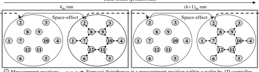
Fig. 1 is the concept of 2D-PPC. For easy interpretation and maximum coverage with minimum measurements, this study assumes that the wafer has 12 measurements in the triangular coordinate (hexagonal grids). In Fig. 1, measurements are divided into two circles, measurements 1-6 are in the outer circle and the others are in the inner circle, and the arrow means that measurements affect others nearby. In addition, after forecasting intercept of measurements independently by

the time-effect (one-dimensional) controller, the

two-dimensional intercept predictor, which is the realization of space effect controller, modifies the forecasting intercept of the 1D controller to forecast intercept of the next run. In other words, 2D-PPC interlaces time and space effects at a run. Then, the process recipe for the next run can be obtained by process models of every measurement.

We conducted simulations to compare the performance of PPC controllers with and without 2D-PPC. The two dimensional anthropogenic disturbance is conducted from DOE data of CMP process and the candidate controllers are examined by average and standard deviation within a wafer in the simulations. The controller parameters such as the propagation parameters of PPC and 2D-PPC were obtained from training data with minimum sum square error. The simulation results show 2D-PPC, which involves space-effect, can improve the ones of time-effect controllers.

The rest of this paper is organized as follows: the two dimensional digital pheromone infrastructure; the 2D-PPC controller structure; simulation results; conclusion and future works

II. THETWO-DIMENSIONAL DIGITAL PHEROMONE

INFRASTRUCTURE

The concept of the space-effect 2D-PPC comes from the appearance that a measurement in a wafer will be affected by its nearby measurements within the same wafer in semiconductor fabrication. This section will introduce the two dimensional digital pheromone infrastructure which includes pheromone basket pheromone states, transition parameters and transition functions.

A. Pheromone Basket

The pheromone basket is the pheromone propagation environment. The “two-dimensional” PPC is named by the shape of pheromone basket being a two-dimensional plane. The environment of two dimensional digital pheromone infrastructure is a tuple <B, N>, where B is a finite set of

Two-Dimensional Pheromone Propagation Controller

(2)

positions

2 : 2

m

b B m 1, 2, … , M2within the pheromone

basket with size M2 and the subscript 2 means

two-dimensional. Specifically,

2

m

b of 2D-PPC maps

positions at the space and does not map the intercept of the specific run at the same measurement like PPC. Then,

2

( _m )

N b B is a finite set of neighbors of

2

m

b and

2

( m )

N b

is the size of

2

( m )

N b . In addition, this study assumes that

2

m

b

will accept propagation inputs from

2

( _m )

N b without

preconditions.

8 9

10

1 7

12 11

2 3

6 5

4

8 9

10

1 7

12 11

2 3

6 5

4

kthrun (k+1)thrun

8 9

10

1 7

12 11

2 3

6 5

4

8 9

10

1 7

12 11

2 3

6 5

4

8 9

10

1 7

12 11

2 3

6 5

4

Forecast disturbance at a measurement position within a wafer by 1D controller.

Modify forecasting disturbance of 1D controller by 2D intercept predictor. Time-effect (process run)

Measurement positions

Space-effect Space-effect

Fig. 1. Concept of space-time-effect 2D-PPC.

Then, the pheromone basket is initially empty, and then fills with M2intercepts within the same wafer at each time

stamp (or run). The external input of two dimensional

pheromone basket is a finite set

2

2( , ) { ( ,2 m, ) ( , ) : 2

R k i r k b i L L m 1, 2, … , M2}, where

k 1, 2, … , is the run number of the manufacturing process,

i is the number of iterations (or propagations) in the transition functions, and L is the global limit of the external inputs in the environment <B, N>. Since the external input is the initial condition for launching transition functions of pheromone propagation,

2

2( , m , 0)

r k b maps to the

intercepts of position

2

m

b at the run k and

2

2( , m , )

r k b i is 0

when iis larger than 0.

A. Pheromone States

Like [11]-[12], the states in the two dimensional pheromone basket <B, N> are Q k i₂( , ) and S k i₂( , ), where

2

2( , ) { ( ,2 m, ) : 2

Q k i  q k b i  m 1, 2, … ,M2} is a finite set

of the propagated inputs at run k and iteration i, and

2

2( , ) { ( ,2 m, ) : 2

S k i  s k b i  m 1, 2, … , M2} is a finite set

of the aggregated pheromones at run k and iteration i. Therefore,

2

2( , m , )

q k b i is regarded as the propagated input

from

2

( m )

N b to

2

m

b at iteration i and run k . Similarly,

2

2( , m , )

s k b i is regarded as the aggregated pheromone of

2

m

b

at iteration iand run k. Then, Q k₂( , 0)0 and S k₂( , 0)0 are assumed to be the initial conditions. While launching transition functions as shown in the following sections,

2( , )

Q k i disseminates pheromones and S k i₂( , ) aggregates pheromones simultaneously.

B. Pheromone Transition Parameters

By [11]-[12], two transition parameters of the two-dimensional digital pheromone infrastructure are the

evaporation parameter E2∈(0,1] and the propagation

parameter F2∈[0,1). In 2D-PPC, the propagation parameter

F2 describes the effect of a measurement on other nearby

measurements within the same wafer, and the evaporation

parameter E2 indicates that the importance of the

measurement data will “evaporate” with time. Because measurements within a chamber at a time stamp can be treated as a non-dissipative system, the modified pheromone infrastructure uses E2= 1 in a small pheromone basket [12].

C. Transition Functions

Reference [12] modified transition functions of digital pheromone infrastructure [11] to erase the boundary effect for developing PPC. This section will correct the propagation-out ratio at the frontier points of a plane pheromone basket to erase the boundary effect.

For interpreting the interactions easily and obtaining maximum coverage with minimum measurements, the authors employ triangular grids with M2= 12. The layout of the 12

measurements is shown in Fig. 1. The propagation-out ratio at the frontier points of Fig. 1 needs to modified from

2

2/ ( m')

F N b [11] or F₂ (2F₂) [12] to F₂ (3 2 F₂) .

Then, the transition functions become

2

2 2

2

2 2

2

2 2

2

2 2

2 2 2

2 2

( , , 1)

( , , ) (1 )( ( , , )

3 2

( , , )), if 1, 2,...6

( , , ) (1 )( ( , , )

( , , )), if 7,8,...,12

m

m m

m

m m

m

s k b i

F

s k b i r k b i

F

q k b i m

s k b i F r k b i

q k b i m

(1)

2

2 2

2

2 6 2 6 2

2

2 6 2 6

2

2 1 2 1

2

2 1 2 1 2

( , , 1)

( ( , , ) ( , , )), if 1, 2,..., 6

3

( ( , , ) ( , , ))

3 2

( ( , , ) ( , , ))

3

( ( , , ) ( , , )) if 8, 9,...,11

3 m

m m

q k b i F

r k b i q k b i m

F

r k b i q k b i

F F

r k b i q k b i

F

(3)

2 2

2 6 2 6

2

2 1 2 1

2

2 12 2 12 2

2

2 6 2 6

2

2 7 2 7

2

2 1

( ( , , ) ( , , )) 3 2

( ( , , ) ( , , )) 3

( ( , , ) ( , , )), if 7 3

( ( , , ) ( , , )) 3 2

( ( , , ) ( , , )) 3

( ( , , ) 3

m m

m

F

r k b i q k b i

F F

r k b i q k b i

F

r k b i q k b i m

F

r k b i q k b i

F F

r k b i q k b i

F

r k b i

− −

+ +

− −

−

+ −

+ +

+ + =

+ −

+ +

+

2

2( , m 1, )), if 2 12

q k b − i m

⎧⎪⎪ ⎪⎪ ⎪⎪ ⎪⎪ ⎪⎪ ⎪⎪ ⎪⎪ ⎪⎪ ⎪⎪⎪ ⎨⎪ ⎪⎪ ⎪⎪ ⎪⎪ ⎪⎪ ⎪⎪ ⎪⎪ ⎪⎪

⎪ + =

⎪⎪⎪⎩

(2)

The final propagation results of (1) and (2) can be obtained analytically by final value theorem. For example, if M2 is 12, the final propagation results at bm₂ is

[

]

2 2 2 2

2 2,1, 2,2, 2,12,

T

2 1 2 2 2 12

( , , )

( , ,0) ( , ,0) ( , ,0)

m m m m

s k b P P P

r k b r k b r k b

⎡ ⎤

∞ = ⎢⎣ ⎥⎦

i (3)

where P_2,1,m₂ , P2,2,m2 , … , and P2,12,m2 are the quantity of

positions 1-12 affecting position bm₂ within the

two-dimensional pheromone basket and the values of P_2,1,_m₂, 2

2,2,m

P , … , and

2 2,12,m

P are function of F2.

III. TWO-DIMENSIONAL PHEROMONE PROPAGATION

CONTROLLER

Relative to the food trail pheromones in the nature, the 2D-PPC employs “intercept pheromones” within the same wafer in the manufacturing process. The intercept pheromone assumes that the intercept of a measurement will affect others nearby within the same wafer at a run and the space-effect will maintain to affect the next wafer. So, the authors conduct 2D-PPC by interlacing space-effect controller and the traditional time-effect controller, such as PPC, in pairs.

A. Plant

The plant is the process model in a simulation or in a real system, which can be obtained by the linear regression model. This study assumes the process has 12 outputs and each output has its own disturbance and process gain. In addition, considering CMP process, pressure from inner and outer pad of wafer carrier are two inputs of the plant and measurements at the same circle has the same process gain. The demonstrated MIMO plant is

k k k

Y+1= + ⋅α β X +ε+1 k = 0, 1, 2, … (4)

where

1, 1 2, 1 12, 1

T

k k k k

Y+1= ⎣⎡Y + Y + Y +⎤⎦

[

1 2 12

]

T

α= α α α

T 1,1 2,1 12,1

1,2 2,2 12,2

β β β

β

β β β

⎡ ⎤

⎢ ⎥

= ⎢_⎣ ⎥_⎦

1,

2,

k k

k

X X

X

⎡ ⎤ ⎢ ⎥ = ⎢_⎣ ⎥_⎦

and 1, 1 2, 1 12, 1

T

k 1 k k k

ε₊ _{= ⎣}⎡ε ₊ ε ₊ ε ₊⎤_⎦ .

In addition, Yk+1 are measurements at the end of run k; Xk

are two recipes (inputs) of run k; α are initial intercepts of

the process; β are system gains of run k; εk+1 are disturbances, which include noise and uncontrolled terms of run k + 1.

B. The One-Dimensional Controller

The one-dimensional controller is the traditional time effect controller, such as EWMA, double EWMA, PPC, and so on. Specifically, the one-dimensional controller of 2D-PPC control measurements independently in this study. For implementation, this study employs PPC [12] as the one-dimensional controller and the forecast intercept of measurement point m2 at run k + 1 becomes

2, 1 2,M1 2,M1 1

2 2

2 ( ) ( )

( , 0) ( ), 1, 2, ... ,

m k m m

T

m m m

v k v k

R_1, ₂ k P_1, ₂_, ₂ k m M

ε ₊ = ⋅ − ₋

= ⋅ = (5)

where

2 2 1 2 1

1, 1 1, 1, M

( , )

( , , )_m _m ( , _m, ) _m ( , , )T R k i

r k b i r k b i r k b i

2 1,m

⎡ ⎤

= ⎢_⎣ ⎥_⎦

is the external inputs of the measurements, m2, at the pheromone basket of PPC with size M1 along time axis and

2 1 2 1 1 2 1 1

2 1 2 1 2 1

1, , (M ) , (M )

1 1 1

1, , ,

1 1 1

ˆ ( , ,0)

1, ... , , if ˆ

( , ,0)

1, ... , , if

m m m k m m k m

m m m m m m

r k b e

m M k M

r k b e

m M k M

ε

− − − −

⎧ = −

⎪⎪

⎪⎪ _∀ ₌ _>

⎪⎪

⎨⎪ = −

⎪⎪

⎪⎪ ∀ = ≤

⎪⎩

where εˆm m₂, ₁ is forecast intercept of PPC at m2 position and m1 run;em m₂, ₁ is the process error at m2 position and m1 run. In

addition, P1,m m2, 2( )k , which varies with the size of the one-dimensional pheromone basket M1, means measurement

m2 affects m2 itself by one-dimensional controller and is an algebraic expression of the propagation parameter of PPC at

m2, F1,m₂.

C. The Two-Dimensional Intercept Predictor

The two-dimensional intercept predictor is the novel space effect controller, which modifies the forecasting intercepts obtained from the one-dimensional controller. The input of two-dimensional pheromone basket is the forecasting intercepts of the one-dimensional controller.

2 2

2 1 2 2 M

1, 1 , 1 , 1

( ,0) ( , ,0) ( , _m ,0) ( , ,0)T

T

k m k M k

R k₂ r k b r k b r k b

ε ₊ ε ₊ ε ₊

⎡ ⎤

= ⎢_⎣ ⎥_⎦

⎡ ⎤

= ⎢⎣ ⎥⎦

(6) The forecast intercept at run k + 1, εˆk 1₊ , can be obtained

(4)

2 2

2 2 2 2 2 2 2

2 ₂ ₂ ₂ ₂ ₂ ₂

2,1,1 2,2,1 2, ,1 2, ,1

1, 1

2, 1 2,1,2 2,2,2 2, ,2 2,M ,2

, 1 2,1, 2,2, 2, , 2, ,

, 1 _2,1, _2,2, _2, _, _2, _,

ˆ ˆ

ˆ

m M

k

k m

m k _m _m _{m m} _M _m

M k M M m M M M

P P P P

ε ε

ε

ε +

+

⎡ ⎤

⎡ ⎤ _⎢ ⎢ ⎥ _⎢ ⎢ ⎥ _⎢ ⎢ ⎥ _⎢ ⎢ ⎥ _⎢ ⎢ _{⎥ = ⎢} ⎢ ⎥ _⎢ ⎢ ⎥ _⎢ ⎢ ⎥ _⎢ ⎢ ⎥ _⎢ ⎢ ⎥ _⎢ ⎢ ⎥ _⎢ ⎣ ⎦ ⎣

2

1, 1

2, 1

, 1

k

m k

M k ε ε

ε

ε +

+

⎡ ⎤ ⎥ ⎢ ⎥ ⎥ ⎢ ⎥ ⎥ ⎢ ⎥ ⎥ ⎢ ⎥ ⎥ ⎢ ⎥ ⎥ ⎢ ⎥ ⎥ ⎢ ⎥ ⎥ ⎢ ⎥ ⎥ ⎢ ⎥ ⎥ ⎢ ⎥ ⎥ ⎢ ⎥ ⎥ ⎣ ⎦ ⎦

where the values of P_2,1,1, P2,2,1, … , and

P

2,M M2, 2 are function of F2. If F2 is 0, the two-dimensional intercept predictor does not modify the forecasting intercept of the one-dimensional controller. In addition, the propagation result approaches the mean of the external inputs as F2 approaches unity.

D. Recipe Generator

The recipe generator generates the recipe of the process for the next run. We use the linear regression model to produce

ˆ

ˆ _k ˆ_k

T= + ⋅α β X ₊₁+ε ₊₁ (7)

where X_k₊₁∈ℜ , which is a 2 × 1 matrix in this study, is the recipe (input) of run k + 1, αˆ is the estimator of the initial

intercept α , βˆ is the estimator of the system

β

(model gain). Then, the recipe for run k + 1 is

1

1 (ˆ ˆT ) ˆT( ˆ ˆ )

k k

X ₊ = β β −β T− −α ε₊₁ (8) where αˆ and βˆ are obtained from the linear regression model of the off-line DOE and are not equal to the process parameters α and _β; the parameter εˆ_k₊₁ comes from (7), and T is the given target values of measurements within a wafer.

E. The Two-Dimensional Propagation Parameter Tuner

This section proposes two strategies for tuning the two-dimensional propagation parameter F2. The first strategy uses historical (or training) data and examines all possible F2 values to obtain the best fixed propagation parameter, F₂,

with minimum mean square error:

2 2

2 , '

'

min( m k)

F k m

F ≅

∑∑

e (10)

where k′ is the index of the training data. Then, F₂ is used

in the testing data.

IV. SIMULATION RESULTS

The simulation settings included the following: the process model α and _β were

[

]

[

]

1 6 7 12

6700.26 6700.26 4304.63 4304.63

T

α= α α α α

=

and

1,1 6,1 7,1 12,1

1,2 6,2 7,2 12,2

1356.63 1356.63 85.54 85.54

1182.19 1182.19 1458.8 1458.8

T

β β β β

β

β β β β

⎡ ⎤

⎢ ⎥

= ⎢_⎣ ⎥_⎦

⎡− − ⎤

⎢ ⎥

= ⎢_⎣ ₋ ₋ ⎥_⎦

the initial input was [1, 0], the process target T was 4500 nm,

and the offset of controller model (αˆ, ˆβ) will be specified in the beginning of following section respectively. Two performance indices to evaluate the output performance: average (Ave.) and standard deviation (Std.) of the simulated data.

A. Performance Comparison with and Without 2D-PPC

This section compares output performance of nine candidate controllers with model mismatch ξ=1.1. The fixed optimal 1D/2D propagation parameter or weights of the other controllers were obtained using the minimum mean square error from 27 sets of anthropogenic disturbance and one set of anthropogenic disturbance is shown in Fig. 2. The simulation results are listed at Table I. In Table I, the output performance of PPC with 2D-PPC is better in both average Ave. and Std. within a wafer than the one of using PPC alone.

0

10 20

30

0 10 20 30 -3000 -2000 -1000 0 1000

D

isturb

ance (nm

)

Position (Y-axis) Position (X-axis)

Fig. 2. One set of anthropogenic disturbance.

TABLE I: SIMULATION RESULTS WITH ξ=1.1.

PPC PPC with 2D-PPC

Average Ave. within a wafer (nm) 4368.67 246.21

Average Std. within a wafer (nm) 4435.31 220.91

Improvement (%) 50.7 10.3

V. CONCLUSION

(5)

ACKNOWLEDGMENT

The authors would like to thank the National Science Council of the Republic of China for financially supporting this paper under Contract NSC 100-2221-E-009-063-MY2.

REFERENCES

[1] E. Sachs, A. Hu, and A. Ingolfsson, “Run by run control: Combining

SPC and feedback control,” IEEE Trans. Semicond. Manuf., vol. 8, pp. 26-43, Feb. 1995.

[2] J. A. Stefani, S. Poarch, S. Saxena, and P. Mozumder, “Advanced

process control of a CVD tungsten reactor,” IEEE Trans. Semicond. Manuf., vol. 9, no. 3, pp. 366-383, 1996.

[3] J. Wang, Q. P. He, S. J. Qin, C. A. Bode, and M. A. Purdy, “Recursive

Least Square Estimation for Run-to-Run Control with Metrology Delay and Its Application to STI Etch Process,” IEEE Trans. Semicond. Manuf., vol. 18, pp. 309-319, May 2005.

[4] A. Chen and R. S. Guo, “Age-based double EWMA controller and its

application to CMP processes,” IEEE Trans. Semicond. Manuf., vol. 14, no. 1, pp. 11-19, Feb. 2001.

[5] N. S. Patel and S. T. Jenkins, “Adaptive optimization of run-to-run

controllers: The EWMA example,” IEEE Trans. Semicond. Manuf., vol. 13, pp. 97-107, 2000.

[6] E. D. Castillo, “Long run and transient analysis of a double EWMA

feedback controller,” IIE Trans., vol. 31, no. 12, pp. 1157-1169, 1999.

[7] A. C. Lee, Y. R. Pan, and M. T. Hsieh, “Output Disturbance Observer

Structure Applied to Run-to-Run Control for Semiconductor

manufacturing,” IEEE Trans. Semicond. Manuf., vol. 24, no. 1, pp.

27-43, Feb. 2011.

[8] J. H. Chen, T. W. Kuo, and A. C. Lee, “Run-by-run process control of

metal sputter deposition: combining time series and extended Kalman filter,” IEEE Trans. Semicond. Manuf., vol. 20, no. 3, pp. 278-285, 2007.

[9] C. F. Wu, C. M. Hung, J. H. Chen, and A. C. Lee, “Advanced Process

Control of the Critical Dimension in Photolithography,” Int. J. Precis. Eng. Manuf., vol. 9, no. 1, pp. 12-18, 2008.

[10] T. W. Kuo and A. C. Lee, “Assessing Measurement Noise effect in

Run-to-Run Process Control: Extends EWMA Controller by Kalman

Filter,” Int. J. Automation and Smart Technology, vol. 1, no. 1, pp.

67-76, Sep. 2011.

[11] S. Brueckner, “Return from the Ant: Synthetic Ecosystems for

Manufacturing Control,” Ph.D. dissertation, Humboldt University of Berlin, 2000.

[12] D. S. Lee and A. C. Lee, “Pheromone Propagation Controller: the

Linkage of Swarm Intelligence and Advanced Process Control,” IEEE Trans. Semicond. Manuf., vol. 22, no. 3, pp. 357-372, Aug. 2009.

Der-Shui Lee received the B.S. degree in mechanical engineering from the Nation Chung-Hsing University, Tai-Chung, Taiwan, in 1997 and the M.S. degree in mechanical engineering from the National Chiao-Tung University, HsinChu, Taiwan, in 1999 and the Ph.D. degree in 2012 from National Chiao-Tung University in mechanical engineering, HsinChu, Taiwan. After graduation, since 2000, he served as an Assistant Researcher in Chung-shan institute of Science and Technology (CSIST). His research interests include run-to-run (R2R) process control, swarm intelligence, and decision support system.

An-Chen Lee received the B.S. and M.S. degrees in Power Mechanical Engineering from National Tsing-Hua University, Hsinchu, Taiwan, R.O.C. and the Ph.D. degree in 1986 from University of Wisconsin-Madison in Mechanical Engineering, USA. He is designated as Chair Professor of National Chiao-Tung University and currently a Professor in the department of Mechanical Engineering. His current research interests are CNC machine tool control technology, Magnetic bearing technology, Rotor dynamic and control, and Semiconductor manufacturing process control.