Abstract—With the advent of 3G mobile communication system, the traffic of wired and wireless networks become voice/video - data integrated service. For real time operation of voice and video signals, circuit switch traffic or Markovian traffic is the best fitted but for data traffic where small amount of delay is tolerable, the non-Markovian traffic like service time of general distribution with finite buffer is preferable. In this paper, Markov modulated Poisson process (MMPP) traffic, which is in concise form of Markovian chain, is used for multimedia traffic and M/D/1 traffic of fixed length packet is considered for asynchronous transfer mode (ATM) cell. The combined model becomes MMPP + M/D/1 traffic, which is used to get the probability density function and mean delay of a voice/video-integrated network.
Index Terms— ATM cell, voice-data integrated service, mean delay, moment generating function, non-Markovian traffic.
I. INTRODUCTION
The aim of the 3G mobile network is to provide high speed packet communication for real time operation of voice/video-data integrated traffic [1]-[4]. The circuit switched network can carry the traffic at high bit rates at the expense of working with fixed bandwidths. It is suitable for real-time operation but incurs a huge waste of link capacity/bandwidth for the case of burst traffic or the traffic of variable bit rate. The packet switched network on the other hand offers bandwidth when necessary; for example, asynchronous transfer mode (ATM) offers both high and low bit rates and ensure efficient use of the available bandwidth [5]. The most widely used mathematical model of traffic analysis is the Markovian chain. One of the major drawbacks of Markov chain lies in the incorporation of large number of probability states which complicates the analysis of the traffic parameters of a network. Markov arrival process (MAP) provides an equivalent state transition chain of few probability states with some assumption as discussed in [6]. Teletraffic engineering adopts three most widely used cases of MAP which are as follows: phase-type (PH) Markov renewal process (PH-MRP), Markov modulated Poisson process (MMPP) and batch Markovian arrival process (BMAP).
The MMPP is a doubly stochastic Poisson process where
Manuscript received August 23, 2011; revised November 17, 2011. Anupam Roy and Md. Imdadul Islam are with the Department of Computer Science and Engineering, Jahangirnagar University, Dhaka 1342, Bangladesh. Md. Imdadul Islam works also as an adjunct Professor of Electronics and Communications Engineering Department at East West University, 43 Mohakhali, Dhaka 1212, Bangladesh (e-mail: [email protected]; [email protected]).
M. R. Amin is with the Electronics and Communications Engineering Department, East West University, 43 Mohakhali, Dhaka 1212, Bangladesh (e-mail: [email protected]).
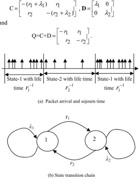
arrival rate of any traffic depends on its probability state which forms a continuous-time Markov chain. In a continuous-time Markov chain, sojourn time/life time in any state i is exponentially distributed with parameter λi. At the end of the sojourn time in state i, a transition takes place to another state or to the same state. The transition may or may not correspond to an arrival. Let us consider the simple case of two-state MMPP, also known as MMPP(2) system, where the arrival rate, λi (i=1, 2) appears alternately with exponentially distributed life time, ri−1(i=1, 2). These are shown in Fig. 1 where the transition between level-1 and level-2 occurs without any arrival. The two-state MMPP is characterized by the matrix pair (Q, D), where Q is the infinitesimal generator matrix and D is the arrival matrix. Here, both Q and D are 2×2square matrices. The generator matrix Q, is expressed as the sum of matrix D and another matrix C; all the off-diagonal elements of C and all the elements of D are nonnegative but the diagonal elements of C are negative:
C ⎥
⎦ ⎤ ⎢
⎣ ⎡
+ − + − =
) (
) (
2 2 2
1 1 1
λ λ
r r
r r
, D ⎥
⎦ ⎤ ⎢ ⎣ ⎡ =
2 1 0
0
λ
λ
and
Q=C+D ⎥
⎦ ⎤ ⎢
⎣ ⎡
− − =
2 2
1 1
r r
r r
.
(a) Packet arrival and sojourn time
(b) State transition chain
Fig. 1. The two-state MMPP.
The n-state MMPP is also characterized by (Q, D), where
now each matrix is an n×n square matrix. The MMPP traffic model is being widely used in recent times as found in the current literature. In [7] the authors deal with waiting time of MMPP(2) traffic, which is applicable to real-time ATM
MMPP+M/D/1 Traffic Model in Video-Data Integrated
Service under ATM System
Anupam Roy, Md. Imdadul Islam, and M. R. Amin, Member, IEEE
1 2
r1
r2 λ2
λ1 State-1 with life
time
r
1−1State-2 with life time
1 2−
r
network. The paper first shows the evaluation technique of the waiting time, based on the generator matrix and Laplace transform [8]. The authors finally suggest an approximate technique following two-term exponential function. The results of both the techniques are found to be very close. In [9], the authors determine the performance of transmission for telemedicine using ATM network. The paper shows the profile of the probability of overflow of queue versus buffer size based on MMPP model. In [10], the authors determine packet loss rate of MMPP/M /1/ K traffic where variable length packet is considered. In [11], performance of voice over Internet (VoIP) traffic is analyzed for a cognitive radio system using a two-state MMPP model.In [12], the average queue length and packet dropping probability of VoIP traffic is analyzed based on statistical multiplexing (talk spurt and silent periods) of two-state MMPP. In [13], authors have claimed the development of an approximate method to evaluate the performance of voice and MMPP video traffic. In [14], constant and variable bit rate traffic is modeled under ATM network and the throughputs for videoconferencing are calculated.
The traffic in circuit switched telecommunications network usually follow exponential arrival and exponential service time distribution like M/M/n/K/N as complete notation. In ATM network, service time of each cell/packet is fixed; hence deterministic service time traffic like M/D/n/K/N is applicable to detect traffic parameters for that network. In case of single server case, ATM traffic can be modeled as M/D/1 of infinite queue which is a special case of M/G/1 [15].
In our present paper, the combined traffic of voice/video and data is modeled by MMPP+M/D/1 based on the concept of MMPP/D/1 and M/G/1 traffic models to determine the mean waiting time of the individual traffic.
The paper is organized as follows: Sec II deals with the traffic model of statistical multiplexing for the case of ATM packet link and its combination with exponential traffic. Section III provides the results of the system model described in Sec. II. Finally, Sec. IV concludes the entire analysis.
II. SYSTEM MODEL
When voice or video signals are sent in packetized form, the system is modeled as of ON-OFF pattern. In case of a single source, the spurt and silence periods are assumed to be exponentially distributed with mean α−1 and β−1
respectively. If the sampling period of voice/video is T (cells / packets are formed for a fixed duration T of the analog signal), then three statistical parameters of the traffic are [16], [17]:
the packet arrival rate,
(
αβ β)
λ
+ =
T , (1) the SCV of inter arrival time,
(
)
(
)
2 22
2 1 1
β α
α
+ − − =
T T
Ca , (2) the skewness of service time,
(
)
(
)
[
]
3/22 2
2
3 3 2
T T
T T T Sk
α α
α α
α −
+ −
= . (3)
The two-phase MMPP parameters are determined as [11], [17]:
⎪ ⎪ ⎩ ⎪ ⎪ ⎨ ⎧
=
⎟⎟ ⎠ ⎞ ⎜⎜
⎝ ⎛
+ −
=
⎟⎟ ⎠ ⎞ ⎜⎜
⎝ ⎛
+ + =
2 ; 1
1 1
1 ; 1
1 1
i E n D
i E n D
ri
λ
λ (4)
⎪⎩ ⎪ ⎨ ⎧
= +
− +
= +
+ + = ′
2 ; 1
1 ; 1
i E n F F n
i E n F F n
i
λ λ
λ λ
λ (5)
where
(
)
1 1
2 2
1
−
− −
+ =
a
H H H
H
C K K
D λ λ λ ,
(
1)
3
2 3 3
. 4 23 2
−
+ − −
=
a
a a k a
C
C C S C D
F ,
and
1
(
1 2)
2F K K
E= HλH + − H λH −λ .
Equations (1)-(5) provide parameters of the MMPP traffic model. Again the actual and virtual waiting time of MMPP/G/1 model as explained in [17] and [18] are:
ρ − + =W 1uh
Wv M , (6) and
(
ρ)
ρ − + =
1 uh W
Wa M , (7) respectively, where WM is the mean waiting time of M/G/1 traffic and is expressed as
(
ρ)
ρλ− =
1
h
WM t . (8) The parameter λt and u are given below in Eqs. (9) and (16) respectively. Now for voice data integrated traffic of MMPP + M/D/1 case, let λpbe the Poisson’s arrival rate of the voice traffic. We have λ1=λ1′+λp and λ2=λ2′ +λp,
where expressions of λ1′ and λ2′ are given by Eq. (5). To determine mean waiting time, we note that
2 1
2 1= r r+r
π ,
2 1
1 2 =r r+r
π ,
and
2 1
1 2 2 1
r r
r r t = λ ++λ
λ . (9) Let us define a function
( )
(
(
)
(
)
)
(
)
(
)
(
1 1)
4 ,2 1
1 1
2 1
2 1 2 2 2
1 1
2 2
1 1
r r r
z r
z
r z r
z z
W
− − − − + − +
+ − + + − =
λ λ
λ λ
( )
{
(
)(
) (
)
}
(
)(
) (
)
{
1}
4 .2 1
1 2 1
2 1 2 2 1 2 1
2 1 2 1
r r r
r z
r r z
z W
− − + − − +
+ + + − =
λ λ
λ λ
(10)
For MMPP/ D/1 model, we have
z=b∗(W(z))=e−hW(z). (11) Solving the above equation, we get the value of z. Let us evaluate the probabilities of transitions P01and P02, we obtain
( )
( )
(
λ λ)( ) (
ρ)
γ −
− −
− −
= 1
1 1 2
2 1
01 W z R z z
P , ρ =λth; (12)
and
P02=1−ρ−P01, (13) where
Rj
( )
z =λj(
1−z)
+rj; j =1, 2. The mean waiting time is
( )
⎟⎟⎠ ⎞ ⎜
⎜ ⎝
⎛ −
+ =
G u W z
Wj πj v λj λt , j =1, 2; (14) where
∑
(
)
=
−
= 2
1
2
j j j t
G π λ λ , (15) and
(
1)(
1 2)
2[
1 01(
1 2)
2 02(
1 1)
]
. 21 rP h r P h
r r
u λ λ
ρ λ
λ − − −
+ −
−
= (16)
Now the mean waiting time of the individual traffic is given by
t D
MMPP W W
W
λ λ λ
′ ′ + ′
= 1 1 2 2
1 /
/ , (17)
where
2 1
1 2 2 1
r r
r r t′= λ′ ++λ′
λ (18) and
2
1 W
W
Wvoice = + . (19)
III. RESULTS
It is to be noted here that the steady state probability states of M/G/1 traffic are given by the following expression ( )
! 1
0
* G z
dz d Lt
j j
j z
j = →
Π ,
where j = 0, 1, 2, 3… and the moment generating function G(z) is expressed in generalized form as
G(z)=(1−a)
{
b*(λ−λz)(z−1)} {
/z−b*(λ−λz)}
. In M/D/1 model, b*(λ−λz)=exp{
−hλ((1−z)}
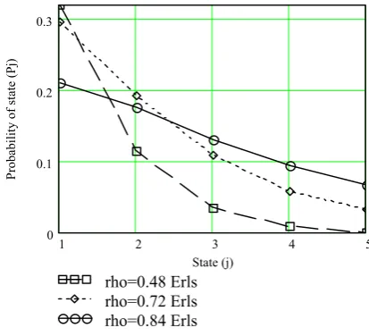
.The detailed derivation of the steady state probability Π*j in terms of the moment generating function G(z) is given in Appendix A.Varying the traffic intensity ρ , the probability of states of the M/D/1 traffic model is plotted in Fig. 2. The tail of the probability density function (PDF) increases with increase in the offered traffic intensity, ρ.
1 2 3 4 5
0 0.1 0.2 0.3
rho=0.48 Erls rho=0.72 Erls rho=0.84 Erls
State (j)
Pr
ob
ab
ility
o
f state (
P
j)
Fig. 2. The probability of state of the M/D/1 traffic.
0.4 0.5 0.6 0.7 0.8 0.9 1 0.04
0.02 0 0.02 0.04
z
f(z)
Fig. 3. Graphical solution of f(z)=z−e−hW( )z .
0 0.1 0.2 0.3 0.4 0.5 0.6 0.7
0.5 1 1.5 2 2.5
Virtual waiting time Actual waiting time Mean waiting time
Traffic intensity (rho)
W
aiting tine
Fig. 4. The variation of virtual, actual and mean waiting time against offered traffic intensity.
0.2 0.4 0.6 0.8 0
0.5 1 1.5 2 2.5
Waiting Time of VIDEO Traffic Waiting Time of Data Traffic
Offered Traffic Intensity (rho) in Erls
Mean wainting time (ms
)
Fig. 5. Waiting time profile of video and data traffic of the combined model.
In the MMPP/D/1 traffic model, the following set of practically realizable traffic parameters are used: λ1 = 0.36 cells/ms, λ2 = 0.2 cells/ms, h = 2ms, r1 = 0.015 and r2 = 0.125. For the above physical parameters, we obtain
(
1r2 2r1) (
/r1 r2)
t = λ +λ +λ = 0.343 cells/ms. Now solving
the relation, f(z)=z−exp{−hW(z)} for the case of deterministic service time, we get z = 0.62. The graphical solution of Eq. (11) is shown in Fig. 3, where z = 0.62 corresponds to the zero crossing point. The variation of virtual, actual and mean waiting time [17], [18] against the offered traffic intensity ρ is shown in Fig. 4, where each of the three parameters rises exponentially with increase in the traffic intensity,ρ .
Let us now go for the combining scheme of M/D/1 and MMPP/D/1, known as MMPP+M/D/1, applicable to voice- data integrated service through ATM network. Let, h = 2.718×10⁻⁶s, T = 3.397×10⁻⁶ s and n = 3, we get the MMPP traffic parameters in per ms as: r1 = 0.414, r2 = 0.071, λb1 = 3.657×10² cells/ms and λb2 = 6.239cells/ms. Therefore, we get, λb = (λb1r2+λb2r1)/(r1+r2) = 58.499cells/ms. Taking λp = 100 cells/ms we can evaluate: λ1 = λb1 + λp = 465.652 cells/ms, λ2 = λb2 + λp = 106.239 cells/ms, λt = (λ1r2 + λ2r1)/(r1 + r2) =158.499 cells/ms and ρ = λth = 0.431 Erls. From the graphical solution of f(z)=z−e−hW
( )
z , shown in Fig. 3, we get z = 0.62. From the expressions of the transition probabilities, given by Eqs. (12) and (13), we obtain
{
( )
( )
}(
) (
{
)( )
}
4
1 2 2
1 01
10 93 . 2
1 /
1
−
× =
− − −
− −
= W z R z r z
P ρ λ λ
and
P02=1−ρ−P01=0.569, where
(
)
[
(
)
(
)
]
(
1)(
)
28.842. 11
2 2 1
1 02 2 2 01 1 2
1 =
+ −
− −
− −
=
r r
h P
r h P
r u
ρ
λ λ
λ
λ
Now the mean, virtual and actual waiting time of Eqs. (6) and (7) are WM=λth2/2(1-ρ) = 1.029E-3 ms, Wa= WM + uh/ρ(1-ρ) = 0.321ms, Wv = WM + uh/(1-ρ) = 0.139ms. The
mean waiting times, Wj (j=1,2), of Eq. (14) are: W1 = P1{ Wv + u(λ1-λt)/G } = 0.1ms and W2 = P2{Wv + u(λ2-λt)/G } = 0.038ms. The individual waiting times are: for video, Wb = (W1 λb1+W2 λb2)/ λb = 0.632 ms and for data Wp = W1+W2 = 0.139 ms.
The variation of the mean waiting time of the video and data traffic is shown in Fig. 5 against the offered traffic. Initially, the waiting time of each of the traffic rises slowly, and after 0.8 Erls, they rise rapidly since packet traffic starts to rise asymptotically there, after ρ = 0.88Erls [16]. When offered traffic tends to be in saturation, i.e., above 0.95 Erls, we find the waiting time to approach infinity since the rate of service falls below the arrival of packets, hence queue will increase continuously.
IV. CONCLUSION
The paper shows the profile of mean waiting time, virtual and actual waiting times of MMPP/D/1 against offered traffic, where all of them are found to be very close to each other and exponentially distributed as is visualized from Fig. 4. Finally, combined model of MMPP+M/D/1 is applied for video-data integrated traffic and waiting time of individual traffic is also evaluated. Both video and data traffic can tolerate the offered traffic below 0.88 Erls/trunk; which satisfies the asymptote of packet traffic. Similar analysis can also be applied in other MAP, like batch arrival process, phase type renewal process along with M/G/1 model to support traffic of variable packet length.
APPENDIX A
In queuing system, moment generating function or z-transformation is used to derive statistical parameters of a network traffic. The moment generating function is defined as [19]:
∑
∞= =
0 ) (
n n nz P z
G ,
which is used in a system of infinite number of probability states. Some properties of the function G(z) are:
∑
∞= = =
0 1 )
1 (
n n P
G ,
∑
∞=
− = =
0
1 1 )
( n
n nz nP dz
z dG
,
∑
∞= =
= =
0 1
] [ )
(
n n z
n E nP dz
z dG
,
( ) [ ] [ ]
0
2
1 2 2
n E n E nP dz
z G d
n n z
− = =
∑
∞= =
,
∑
∞= − =
0 1 )
( n
n n z P z
zG ,
1[ ( ) 0] 0 1
P z G z z P n
n
n = − −
∞
= +
∑
.and j calls arrive during its service time, then the number of calls present at its departure is k+j-1.
Let Π*j is the probability that j calls exist just after departure of a call in M/G/1 system and pj is the probability that j calls arrive during the service time [17].
Therefore, , ... ... ... ... * 1 0 * 1 * 3 2 * 2 1 * 1 * 0 * + + − − − Π + + Π + + Π + Π + Π + Π = Π j k k j j j j j j p p p p p p
which can be compactly written as
1 * 1 1 * 0 * k j
k j k j
j =p Π + p Π
Π
∑
+= − +
; j = 0, 1, 2, … , (A1) where
a j
j j e a
p = −
! . From total probability theorem, we have
( )
( ) ! 0 x dB e j xp j x
j λ −λ
∞
∫
= ,
where B(x) is the service time distribution.
Let the probability generating function of Π*j be G(z), then . ) ( 0 * 1 1 1 0 * 0 * 1 1 1 * 0 0 0 *
∑
∑
∑
∑
∑
∑
∞ = + = − + ∞ = + = − + ∞ = ∞ = Π + Π = ⎪⎭ ⎪ ⎬ ⎫ ⎪⎩ ⎪ ⎨ ⎧ Π + Π = Π = j k jk j k
j j j j k j
k j k
j j j j j j p z p z p p z z z G
Let us consider the second part of the above relation:
∑ ∑
∞ = + = − +Π 0 * 1 1 1 j k jk j k j p z
∑ ∑
∞ = + = − +Π = 0 * 1 1 1 j k jk j k jp z
∑ ∑
∞ = + = − +Π = 0 * 1 1 1 k j kj k j kp
z ; (interchanging the index k and j)
∑ ∑
∞ = ∞ = − +Π = 0 * 1 1k j k j j kp
z ; (Since k varies from 0 to ∞)
∑ ∑
∞ = ∞ = − +Π = 1 * 0 1j k k j j kp z
∑ ∑
∞ = ∞ = − + Π =1 0 1
*
j k k j
k j z p
∑ ∑
∞ = ∞ = ′ ′ − + ′ Π = 1 0 * 1j jk k
p zk j .
Taking, k-j+1=k′ when k=0 and j=1, then k′ = 0-1 + 1 = 0, the above expression can be written as
∑
∞∑
= ∞ = − + Π = 1 0 * 1j jk k
p zk j . Now,
∑
∑ ∑
∞ = ∞ = ∞ = − + Π + Π = 1 0 * 0 * 0 1 ) (j jk k
j j
jp z p
z z
G k j . (A.2)
Again we have
( )
( ) ! 0 x dB e j xp j x
j λ −λ
∞
∫
= , which implies( )
( )
, ) ( ) ( ! ) ( ! 0 0 0 0 0 0∫
∫ ∑
∫ ∑
∑
∞ − ∞ ∞ = − ∞ ∞ = − ∞ = = = = x dB e e x dB e j x z x dB e j x z p z x x z j x j j x j j j j j λ λ λ λ λ λ or∑
∞ ∞∫
− − = = 0 ) ( 0 ) (x dB e pz x z
j j
j λ λ . (A.3)
We know the LST of F(x) as
( ) ( .) 0 *
∫
∞ −= e dF x
f θ θx (A.4)
From (A.3) and (A.4), we have *( ) 0 z b p z j j
j = λ−λ
∑
∞=
. (A.5)
From (A.2) and (A.5), we have
∑
∞∑
= ∞ = − Π + − Π = 1 0 * * *0. ( ) 1
) (
j j k k
p z z z b z
G λ λ j k .
∑
∞ = − Π + − Π = − 1 * * * *0. ( ) 1 ( )
j j
z b
z z
b λ λ j λ λ
⎪⎭ ⎪ ⎬ ⎫ ⎪⎩ ⎪ ⎨ ⎧ Π + Π − =
∑
∞ = − 1 * * 0*( ) . 1
j j
j
z z
b λ λ
{
. ... ... ...}
)
( *0 1* *2 *3 2
* − Π +Π +Π +Π +
=b λ λz z z
⎪⎭ ⎪ ⎬ ⎫ ⎪⎩ ⎪ ⎨ ⎧ Π + Π − =
∑
∞ = − 1 * * 0 1 *( ) j j j z z z zb λ λ
{
*}
0 * 0 1 *( − ) Π + ( )−Π=b λ λz z− z G z ,
{
1 ( )}
( ) ( 1)) ( * 0 1 * 1 * − = − Π − −
⇒G z b λ λz z− b λ λz z− z
{
}
{
( )}
) 1 ( ) ( ) ( 1 ) 1 ( ) ( )( * * *0
{
( )}
) 1 )( ( ) 1 ( )( * *
z b z
z z b a z
G
λ λ λ λ
− −
− − −
=
⇒ [QΠ*0=(1−a).
Now the probability states of M/G/1 are ) ( !
1
0
* G z
dz d Lt
j j
j z
j = →
Π ; j = 0, 1, 2, 3…
In M/D/1 model,b*(λ−λz)=exp
{
−hλ((1−z)}
.REFERENCES
[1] A. C. Clearly and M. Paterakis, “On the voice data integration in third generation wiereless access communication networks”, Euro. Trans. on Telecom. and Related Technol., vol. 5, no. 1, pp. 11-18, Jan-Feb, 1994. [2] N. M. Mitrou, G. L. Lyberopoulos and A. D. Panagopoulou, “Voice
data integration in the air interface of a microcellular mobile communication system”, IEEE Trans. on Veh. Technol., vol. 42, no. 1, pp. 1-13, Feb. 1999.
[3] M. Madhovi, R. M. Edwards and S. R. Cvetkovic, “Policy for
enhancement of traffic in TDMA hybrid switched integrated voice/data cellular mobile communications systems”, IEEE Commun. Lett., vol. 5, no. 6, pp. 242-244, June 2001.
[4] G. Anastrasi, D. Grillo, L. Lenzini and E. Mingozzi, “A bandwidth
reservation protocol for speech/data integration in TDMA-based advanced mobile systems”, Int. J. Wireless Info. Networks, vol. 3, no. 4, pp. 243-252, 1996.
[5] Bing Zheng and Mohammed Atiquzzaman, “Traffic Management of
Multimedia over ATM Networks”, IEEE Commun. Magazine, pp.33-38, January 1999.
[6] Sang H. Kang, Yong Han Kim, Dan K. Sung and Bong D. Choi, “An application of Markovian Arrival Process (MAP) to modeling superposed ATM cell stream”, IEEE Trans. Commun., vol. 50, no. 4, pp. 633-642, April 2002.
[7] Sang H. Kang, Dan K. Sung and Bong D. Choi, “An Empirical Real-Time Approximation of Waiting Time Distribution in MMPP(2)/D/1”, IEEE Commun. Lett., vol. 2, no. 1, pp. 17-19, Jan. 1998.
[8] D. M. Lucantoni, “New results on the single server queue with a batch Markovian arrival process”, Commun. Statist. Stochastic Models, vol. 7, no. 1, pp. 1–46, 1991.
[9] J. P. Dubois, and H. M. Chiu, “High Speed Video Transmission for Telemedicine using ATM Technology”, World Academy of Science, Engineering and Technology 12, pp. 103-107, 2005.
[10] L. P Raj Kumar, K. Sampath Kumar, D. Mallikarjuna Reddy, Malla Reddy Perati, “Analytical Model for Loss and Delay Behavior of the Switch under Self-Similar Variable Length Packet Input Traffic”, IAENG Int. J. Computer Science, vol. 38, no. 1, pp. 26-31, Feb. 2011. [11] Howon Lee and Dong-Ho Cho, “VoIP Capacity Analysis in Cognitive
Radio System”, IEEE Commun. Lett., vol. 13, no. 6, pp. 339-395, June 2009.
[12] Jae-Woo So, “Performance Analysis of VoIP Services in the IEEE 802.16e OFDMA System With Inband Signaling”, IEEE Trans. Vehi. Technol., vol. 57, no. 3, pp.1876-1986, May 2008.
[13] T.C. Wang, J. W. mark, K.C. Chua, “Delay performance of voice and MMPP video traffic in cellular wireless ATM network”, IEE Proc. Commun., vol. 148, no. 5, pp. 302-309, Oct. 2001.
[14] Kyoko Yamori and Haruo Akimaru, “Optimum Design of Videoconferencing Systems over ATM Networks”, Electronics and Communications in Japan, Part 1, pp. 33-40, vol. 85, no. 6, 2002. [15] Md. Imdadul Islam, M. F. K. Patwary and M.R. Amin, “Cost
Optimization of Alternate Routing Network of M/G/1(M) Traffic”, The Mediterranean Journal of Electronics and Communications, vol.6, no. 1, pp. 190-195, 2011.
[16] Nogueira, P. Salvador, R. Valadas, “Fitting Algorithms for MMPP ATM Traffic Models”, Proc. of the Broadband Access Conference, Cracow, Poland, October 11-13, 1999, pp. 167-174
[17] Haruo Akimaru and Konosuke Kawashima, “Teletraffic Theory and Applications”, Springer-Verlag, Berlin, 1993.
[18] T. Okuda, H. Akimaru, and M. Sakai, “A simplified performance evaluation of packetized voice system”, IEICE, vol. E73, no. 6, 1990. [19] Mischa Scwartz, “Telecommunication Networks: Protocol, Modeling
and Analysis”, Prentice Hall; 1987.
Anupam Roy has completed B.Sc Engineering in
Computer Science and Engineering from Jahangirnagar University, Savar, Dhaka, Bangladesh in 2007. He is now pursuing M.Sc Engineering at the same department. He worked few months as a General Software Developer in MFASIA LTD (A joint venture company between Bangladesh and England) and Java Programmer in ATI LTD, Dhaka, Bangladesh. He is now working as a Programmer in BJIT LTD (A joint venture company between Bangladesh and Japan), Dhaka, Bangladesh.
Md. Imdadul Islam has completed his B.Sc. and
M.Sc Engineering in Electrical and Electronic Engineering from Bangladesh University of Engineering and Technology, Dhaka, Bangladesh in 1993 and 1998 respectively and has completed his Ph.D degree in 2010 from the Department of Computer Science and Engineering, Jahangirnagar University, Dhaka, Bangladesh in the field of network traffic engineering. He is now working as a Professor at the Department of Computer Science and Engineering, Jahangirnagar University, Savar, Dhaka, Bangladesh. Previously, he worked as an Assistant Engineer in Sheba Telecom (Pvt.) LTD (A joint venture company between Bangladesh and Malaysia, for Mobile cellular and WLL), from Sept'94 to July'96. He has a very good field experience in installation of Radio Base Stations and Switching Centers for WLL. His research field is network traffic, wireless communications, wavelet transform, OFDMA, WCDMA, adaptive filter theory, ANFIS and array antenna systems. He has more than hundred research papers in national and international journals and conference proceedings.
M. R. Amin received his B.S. and M.S. degrees in
Physics from Jahangirnagar University, Dhaka, Bangladesh in 1984 and 1986 respectively and his Ph.D. degree in Plasma Physics from the University of St. Andrews, U. K. in 1990. He is a Professor of Electronics and Communications Engineering at East West University, Dhaka, Bangladesh. He served as a Post-Doctoral Research Associate in Electrical Engineering at the University of Alberta, Canada, during 1991-1993. He was an Alexander von Humboldt Research Fellow at the Max-Planck Institute for Extraterrestrial Physics at Garching/Munich, Germany during 1997-1999.