Satellite derived light extinction coefficient and its impact on thermal structure simulations in a 1 D lake model

www.hydrol-earth-syst-sci.net/21/377/2017/ doi:10.5194/hess-21-377-2017

© Author(s) 2017. CC Attribution 3.0 License.

Satellite-derived light extinction coefficient and its impact on

thermal structure simulations in a 1-D lake model

Kiana Zolfaghari, Claude R. Duguay, and Homa Kheyrollah Pour

Interdisciplinary Centre on Climate Change and Department of Geography & Environmental Management, University of Waterloo, Waterloo, Canada

Correspondence to:Kiana Zolfaghari ([email protected])

Received: 17 February 2016 – Published in Hydrol. Earth Syst. Sci. Discuss.: 24 February 2016 Revised: 1 December 2016 – Accepted: 8 December 2016 – Published: 24 January 2017

Abstract. A global constant value of the extinction coeffi-cient (Kd) is usually specified in lake models to parame-terize water clarity. This study aimed to improve the per-formance of the 1-D freshwater lake (FLake) model using satellite-derived Kd for Lake Erie. The CoastColour algo-rithm was applied to MERIS satellite imagery to estimate Kd. The constant (0.2 m−1) and satellite-derivedKdvalues as well as radiation fluxes and meteorological station obser-vations were then used to run FLake for a meteorological station on Lake Erie. Results improved compared to using the constantKdvalue (0.2 m−1). No significant improvement was found in FLake-simulated lake surface water tempera-ture (LSWT) whenKdvariations in time were considered us-ing a monthly average. Therefore, results suggest that a time-independent, lake-specific, and constant satellite-derivedKd value can reproduce LSWT with sufficient accuracy for the Lake Erie station.

A sensitivity analysis was also performed to assess the impact of various Kd values on the simulation outputs. Re-sults show that FLake is sensitive to variations inKdto es-timate the thermal structure of Lake Erie. Dark waters re-sult in warmer spring and colder fall temperatures compared to clear waters. Dark waters always produce colder mean water column temperature (MWCT) and lake bottom water temperature (LBWT), shallower mixed layer depth (MLD), longer ice cover duration, and thicker ice. The sensitivity of FLake to Kd variations was more pronounced in the simu-lation of MWCT, LBWT, and MLD. The model was par-ticularly sensitive to Kd values below 0.5 m−1. This is the first study to assess the value of integrating Kd from the satellite-based CoastColour algorithm into the FLake model. Satellite-derivedKdis found to be a useful input parameter

for simulations with FLake and possibly other lake models, and it has potential for applicability to other lakes whereKd is not commonly measured.

1 Introduction

lim-ited to 40–60 m depth; Kourzeneva et al., 2012a), located in both temperate and warm climate regions (Kourzeneva, 2010; Martynov et al., 2010, 2012; Mironov, 2008; Mironov et al., 2010, 2012; Samuelsson et al., 2010; Kourzeneva et al., 2012a, b).

One of the optical parameters required as input in the FLake model is water clarity. This variable is considered as an apparent optical property and is parameterized using the light extinction coefficient (Kd) to describe the absorption of shortwave radiation within the water body as a function of depth (Heiskanen et al., 2015). A global constant value of Kdis usually used to run lake models, including FLake. For example, Martynov et al. (2012) coupled FLake with the Canadian Regional Climate Model (CRCM) by specifying a Kd value equal to 0.2 m−1 (A. Martynov, personal com-munication, 2015) for all North American lakes, including Lake Erie, for the years 2005–2007. Heiskanen et al. (2015) evaluated the sensitivity of two 1-D lake models, LAKE and FLake, to seasonal variations and the general level of Kd for simulating water temperature profiles and turbulent fluxes of heat and momentum in a small boreal Finnish lake. Modeled values were compared to those measured for the lake during the ice-free period of 2013. The study found a critical threshold for Kd (0.5 m−1) in 1-D lake models. Heiskanen et al. (2015) concluded that for too-clear waters (Kd<0.5 m−1), the model is much more sensitive toKd. The study recommends a global mapping ofKdto run the FLake model for regions with clear waters (Kd<0.5 m−1) for fu-ture use in NWP models. The authors also suggest that this global mapping can be time-independent (i.e., with a con-stant value per lake).

The global mapping of Kd can be derived from satellite imagery. Potes et al. (2012) used empirically derived water clarity from space-borne medium resolution imaging spec-trometer (MERIS) measurements to test the sensitivity of FLake to this parameter. The sensitivity analysis was con-ducted using two Kd values, representing the expected ex-treme water clarity cases for their study (1.0 m−1 for clear water and 6.1 m−1for dark water). The importance of lake optical properties was evaluated based on the evolution of LSWT and heat fluxes. Their results showed that water clar-ity is an essential parameter affecting the simulated LSWT. The daily mean LSWT increased from 1.2◦C in clear wa-ter to 2.4◦C in dark water (Potes et al., 2012). Water clarity measurements are included in water quality monitoring pro-grams; however, global measurements of clarity are not yet available. Satellite remote sensing can provide water clarity observations to the modeling communities at higher spatial and temporal resolutions, to fill the gap of field measure-ments.

In recent years, a number of algorithms have been devised to retrieve different water optical parameters, including wa-ter clarity, from satellite observations for coastal (ocean) and lake waters (Attila et al., 2013; Binding et al., 2007; Bind-ing et al., 2015; Olmanson et al., 2013; Potes et al., 2012;

Wu et al., 2009; Zhao et al., 2011; Zolfaghari and Duguay, 2016). Turbid inland and coastal waters are optically more complex compared to open ocean, and large optical gradients exist. There is more than only one component (phytoplank-ton species, various dissolved and suspended matters with non-covarying concentrations) in coastal waters and lakes that determines the variability of water-leaving reflectance. Considering this complexity, the development of algorithms for coastal waters and lakes is more challenging. MERIS, which operated from March 2002 to April 2012, collected data from the European Space Agency’s (ESA) Envisat satel-lite. The spatial resolution and spectral bands settings were carefully selected in order to meet the primary objectives of the mission; addressing coastal monitoring from space. The best possible signal-to-noise ratio, additional channels to measure optical signatures, and the relatively high spa-tial resolution of 300 m are some of the specific instrument characteristics (Ruescas et al., 2014). In 2010, ESA launched the CoastColour (CC) project to fully exploit the potential of MERIS instrument for remote sensing of coastal zone waters. CoastColour is providing a global data set of MERIS full resolution data of coastal zones that are processed with the best possible regional algorithms to produce water-leaving reflectance and optical properties (Ruescas et al., 2014).

The objectives of this study were to: (1) evaluate satellite-derivedKdvalues for a large lake in the Great Lakes region; (2) apply the evaluated satellite-derivedKdin FLake model to investigate the improvement of model performance to re-produce LSWTs, compared to previous studies using a con-stantKdvalue of 0.2 m−1. Therefore, three different values ofKdwere used in the simulations: yearly average, monthly average, and a constant value of 0.2 m−1_{to evaluate the} im-pact of a time-independent, lake-specificKdvalue in simu-lating LSWT; and (3) understand the sensitivity of the FLake model to variations inKd, based on the analysis of simulated LSWT, mean water column temperature (MWCT), lake bot-tom water temperature (LBWT), mixed layer depth (MLD), and water temperature isotherms during the ice-free season on Lake Erie (from April to November). The impact ofKd variations on ice dates (freeze-up, break-up, and duration) and ice thickness was also evaluated.

2 Data and methods

2.1 Study site and station observations

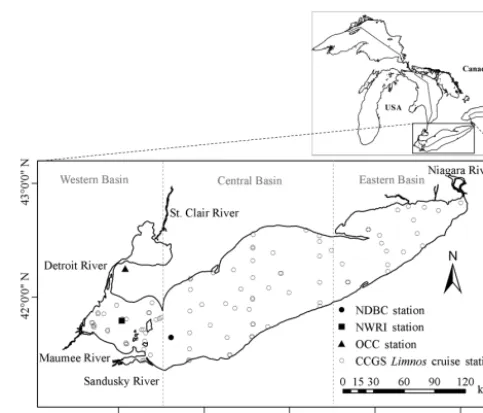
Lake Erie (42◦₁₁0_{N, 81}◦₁₅0_{W; Fig. 1) is a large shallow}

The meteorological forcing variables required for FLake model runs include solar (shortwave) and longwave irradi-ance, air temperature, air humidity, wind speed, and cloudi-ness. These data were collected from different stations shown in Fig. 1. Mean daily air temperature, wind speed and wa-ter temperature measurements were obtained for the years 2003–2012, from the National Data Buoy Center (NDBC) of NOAA, station 45005 (41◦400N, 82◦230W, and depth: 12.6 m). Air temperature is measured 4 m above the water surface and anemometer height is 5 m above the water sur-face to measure the wind speed, whereas the water sursur-face is at 173.9 m above mean sea level. Water temperature is mea-sured at 0.6 m below the water surface. The NDBC station was selected to perform simulations with FLake, since water temperature observations collected at the buoy station can be used to evaluate the model output. The other meteorologi-cal forcing variables required for model simulations at the NDBC station were obtained from nearby stations. Air hu-midity and cloudiness were available in a daily format from the Ontario Climate Center (OCC), Environment and Cli-mate Change Canada (ECCC) for the Windsor station (cli-mate ID: 6139525) (2003–2012). This station is a near-shore station close to the NDBC station. The distance between the OCC and NDBC stations is less than 81 km. Incoming radia-tion flux data were supplied by the Naradia-tional Water Research Institute (NWRI), ECCC, from a station located in the west-ern basin of Lake Erie. Daily shortwave irradiance measure-ments were available only for 2004 and 2008. Therefore, a daily time series of solar irradiance for the entire study pe-riod (2003–2012) was completed for the NDBC station using solar irradiance model data (see Sect. 2.2). Longwave irradi-ance was measured only in 2008 at the NWRI station. An empirical equation (see Sect. 2.2) was therefore employed to obtain longwave irradiance for the full period of study (2003–2012).

FLake requires information on water transparency (down-ward lightKd) as input for model runs. MERIS satellite im-agery was used to deriveKdfor the NDBC station during the study period. The method is described in details in Sect. 2.3. Available Secchi disk depth (SDD) field measurements were collected by ECCC research cruises on board the Canadian Coast Guard shipLimnosand utilized in this study to evalu-ate the sevalu-atellite-derived wevalu-ater clarity. The cruise visited Lake Erie at a total of 89 distributed stations in five different years (September 2004; May, July, and September 2005; May and June 2008; July and September 2011; and February 2012).

2.2 Shortwave and longwave irradiance

The SUNY model, a satellite solar irradiance model, has been developed to exploit Geostationary Operational En-vironmental Satellites (GOES) for deriving solar irradi-ance using cloud, albedo, elevation, temperature, and wind speed observations (Kleissl et al., 2013). The basic princi-ples of solar-irradiance modeling based on inputs from

geo-Figure 1.Maps showing Lake Erie in Laurentian Great Lakes and the location of stations where different parameters were measured. NDBC: National Data Buoy Center. NWRI: National Water Re-search Institute. OCC: Ontario Climate Center. CCGS: Canadian Coast Guard Ship. Vertical dashed lines separate different basins in the lake.

stationary satellites and atmospheric models are described in Kleissl et al. (2013). Data from these sources are used to generate site- and time-specific high-resolution maps of solar irradiance with the SUNY model. The daily mean solar irradiance data for the present study was obtained from the second version of the SUNY model (Version 2.4), available in SolarAnywhere® (https://www.solaranywhere. com). The model provides a gridded data set with a spa-tial resolution of 1/10 of a degree (ca. 10 km). The so-lar irradiance data was extracted from a tile correspond-ing to the NWRI station for 2004 and 2008, when obser-vations were available for evaluation, and also for FLake model run on Lake Erie for the full study period (2003– 2012). There is a strong agreement (R2=0.93) between model-derived and measured solar irradiance at the NWRI station. The SUNY model slightly underestimates obser-vations by 2.18 W m−2 (N=362, RMSE=21.58 W m−2, MBE= −2.18 W m−2,Ia=0.88; see Sect. 2.5 for details).

Longwave irradiance was computed on a daily basis us-ing the equation of Maykut and Church (1973), as imple-mented in the Canadian Lake Ice Model (CLIMo) (Duguay et al., 2003):

E=σ T4 0.7855+0.000312G2.75, (1) whereT is the air temperature at screen height (◦K) andGis the cloudiness in tenth from meteorological stations.

(R2=0.74) with the equation underestimating measured ir-radiance by 0.86 W m−2 _{(N=194, RMSE=17.74 W m}−2_, MBE= −0.86 W m−2_,I

a=0.76). Model-derived incoming shortwave and longwave fluxes were used as input in FLake model simulations for subsequent analyses in the NDBC sta-tion over the 2003–2012 period.

2.3 Satellite-derived extinction coefficient

MERIS operated on-board the ESA Envisat polar-orbiting satellite until April 2012. The sensor was a push-broom imaging spectrometer which measured solar radiation re-flected from the Earth’s surface at high spectral and radio-metric resolutions with a dual spatial resolution (300 and 1200 m). Measurements were obtained in the visible and near-infrared part of the electromagnetic spectrum (across the 390–1040 nm range) in 15 spectral bands during daytime, whenever illumination conditions were suitable, and with a full spatial resolution of 300 m at nadir, with a 68.5◦field of view. MERIS scanned the Earth with a global coverage of every 2–3 days.

In this study, a total of 326 full-resolution archived MERIS images encompassing the NDBC station in Lake Erie were acquired from CC (Version 2) products through the Calvalus on-demand processing service for the period of 2003–2012. The level 2 products are generally geolocated geophysical products and CC Level2W products are the result of in-water processing algorithms to derive optical parameters from the water-leaving reflectance. These parameters include inherent optical properties (IOPs), concentrations of some water con-stituents, and other optical water parameters such as spectral vertical Kd. The IOP parameters are first derived applying two different inversion algorithms: neural network (NN) and quasi-analytical algorithm (QAA). The derived IOPs are then converted to estimate constituents’ concentrations and appar-ent optical properties (AOPs), including diffuseKdfor differ-ent spectral bands applying Hydrolight simulations (Ruescas et al., 2014).

The diffuse Kdproduct (the average value between visi-ble spectral bands) in CC Level2W data was extracted for the pixel at the geographic location of the NDBC station. The satellite-derivedKdvalues were also extracted for pixels on the same day and location as the Limnoscruise stations, to evaluate the CC-derived diffuse Kd values against SDD in situ data collected during Limnos cruises. A valid pixel expression was defined in all pixel extraction steps that ex-cluded pixels with properties listed in Table 1.

2.4 FLake model and configuration

The FLake model is a self-similar parametric representation (assumed shape) of the temperature structure in the four me-dia of the lake including water column, bottom sediments, and the ice and snow. The water column temperature profile is assumed to have two layers: a mixed layer with constant

temperature and a thermocline that extends from the base of mixed layer to the lake depth. The shape of thermocline tem-perature is parameterized using a fourth-order polynomial function of depth that also depends on a shape coefficient CT. The value ofCTlies between 0.5 and 0.8 so that the ther-mocline can neither be very concave nor very convex. FLake has an optional scheme for the representation of bottom sed-iments layer, which is based on the same parametric concept (De Bruijn et al., 2014; Martynov et al., 2012). The system of prognostic equations for parameters is described in Mironov (2008).

The prognostic ordinary differential equations are solved to estimate the thermocline shape coefficient, the mixed layer depth, the bottom, mean and surface water column temper-atures, and also parameters related to the bottom sediment layers (Martynov et al., 2012; Mironov, 2008; Mironov et al., 2010). The same parametric concept is applied for the ice and snow layers, using linear shape functions (Martynov et al., 2012). The mixed layer depth is calculated considering the effects of both convective and mechanical mixing, also accounting for volumetric heating which is through the ab-sorption of net shortwave radiation (Thiery et al., 2014). The non-reflected shortwave radiation is absorbed after penetrat-ing the water column in accordance with the Beer–Lambert law (Gordon, 1989).

Stand-alone FLake simulations were conducted for the NDBC station. The setup condition of the NDBC buoy sta-tion, such as height of wind measurement (5 m), height of air temperature sensor (4 m), and the geographic location and depth of this site were used to configure the model. The mea-sured meteorological parameters and model-derived irradi-ance were also used to force the FLake model. A fetch value of 100 km was used to run all simulations. It was found that there is only a little sensitivity to modifications in this pa-rameter for Lake Erie. The same result was found for Lake Kivu in Thiery et al. (2014). The bottom sediments module was switched off in all simulations and the zero bottom heat flux condition was adopted. The initial temperature value for the upper mixed layer and the lake bottom were 4◦C. Mixed layer thickness had the initial value of 3 m. The simulations were run in a daily time step (using daily forcing data) for 2003–2012.

The ability of FLake to reproduce the observed tempera-ture variations using differentKdvalues was tested by com-paring the simulated LSWT to the corresponding in situ ob-servations in the NDBC station. Also, the model sensitivity to variations in water clarity was assessed by studying the LSWT, MWCT, LBWT, MLD, isotherms, ice phenology, and ice thickness.

2.5 Accuracy assessment

Table 1.Flags of excluded pixels.

Level 1 Level 1P Level 2

Glint_risk Land AOT560_OOR (aerosol optical thickness at 550 nm out of the training range)

Suspect Cloud TOA_OOR (top of atmosphere reflectance in band 13 out of the training range)

Land_ocean Cloud_ambiguous TOSA_OOR (top of standard atmosphere reflectance in band 13 out of the training range)

Bright Cloud_buffer Solzen (large solar zenith angle)

Coastline Cloud_shadow NN_WLR_OOR (water-leaving reflectance out of training range)

Invalid Snow_ice NN_CONC_OOR (water constituents out of training range) MixedPixel NN_OOTR (spectrum out of training range)

C2R_WHITECAPS (risk of white caps)

comprehensive metric that combines the mean and variance of model errors into a single statistic (Moore et al., 2014). The MBE is calculated as the mean of modeled values mi-nus the in situ observations. Therefore, a positive (negative) value of this error shows an overestimation (underestima-tion) of the parameter of interest. Ia is a descriptive mea-sure of model performance. It is used to compare different models and is also modeled against observed parameters.Ia was originally developed by Willmott in the 1980s (Willmott, 1981) and a refined version of it was presented by Willmott et al. (2012). The refined version, which was adopted in this study, is dimensionless and bounded by−1.0 (worst perfor-mance) and 1.0 (the best possible perforperfor-mance). These statis-tical indices are considered to be robust measures of model performance (e.g., Hinzman et al., 1998; Kheyrollah Pour et al., 2012; Willmott and Wicks, 1980).

3 Results and discussion 3.1 Satellite-derivedKd

3.1.1 Variations ofKdat NDBC station

Figure 2 shows the variations of CC-derived Kd for the NDBC station during the full study period (2003–2012). Lake Erie (specifically its shallow regions) is more suscep-tible to re-suspension of bottom sediments compared to the other Great Lakes, which leads to lower water clarity (Bind-ing et al., 2010). The results from apply(Bind-ing the CC algorithm on MERIS satellite imagery shows that the highestKdvalues in the NDBC station occur in the turn-over times in spring and fall. The maximum value ofKdwas 3.54 m−1, estimated in April 2003. A minimum value of 0.58 m−1was estimated in June 2007. The average value ofKdduring the study pe-riod was 0.90 m−1 with a standard deviation of 0.38 m−1. Hence, these values, identified as the average, the lower, and the upper limits of clarity at the NDBC station, were used to carry out a sensitivity analysis with FLake (see Sect. 3.2.2).

Figure 2.Variations of CoastColour-derivedKdfor the selected lo-cation during the study period (2003–2012).

3.1.2 Evaluation of CoastColourKd

The validation of satellite observations against in situ data is important, because the in situ data are still considered as the most accurate measurement of water clarity. The assess-ment of the satellite-derived Kd retrieval reliability highly depends on the comparison with independent in situ SDD measurements. The general form of the relationship between Kdand SDD was established by the pioneer study of Poole and Atkins (1929):

SDD×Kd=K, (2)

whereKis a constant value of 1.7 (Poole and Atkins, 1929). Following this important work, there were other studies that found a high variability of the constant value (K) depend-ing on the type of the lake considered (Koendepend-ings and Ed-mundson, 1991). Armengol et al. (2003) showed thatKdand SDD are negatively correlated and they developed an empir-ical power relation between these two parameters.

0.2, 11, 3.69, and 2.68 m, respectively. CC Level2W satellite products were acquired on the same day as the in situ mea-surements. Applying defined flags produced 49 data pairs (matchup data set) of CC observations of Kd and SDD in situ data that were collected on the same day and location.

The matchup data set was divided into training and test-ing data in 100 iterations. In each iteration, the data used for the equation’s training and evaluation were kept independent, where 70 % of the sample was used for equation calibra-tion and 30 % for evaluacalibra-tion. Ordinary least-square regres-sion was used in the calibration step of each iteration to relate the in situ measurements of SDD to the CC-derivedKd. Lo-cally tuned equations were derived from this step and applied on SDD observations to predictKdin testing matchup data. The statistical parameters of the model performance were derived between the estimated Kd from SDD observations and the paired CC-derived values. These steps were repeated for 100 iterations, and the final statistical indices, slope, and power of the locally tuned equation was reported as the aver-age of those derived over all iterations.

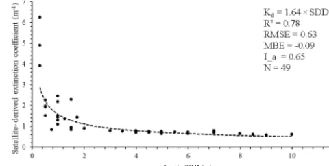
Results from the above procedure show thatKdcan be de-rived from SDD, using the equationKd=1.64×SDD−0.76, with a strong determination of coefficient value (R2=0.78). Arst et al. (2008) obtained a similar regression formula be-tween SDD andKdfor the boreal lakes in Finland and Es-tonia representing different types of water, expanding from oligotrophic to hypertrophic. Because there is a good agree-ment between Kd and the corresponding ones estimated from in-situ-measured SDD (N=49, RMSE=0.63 m−1, MBE= −0.09 m−1,Ia=0.65; Fig. 3), the satellite-derived water clarity measurements were considered to be represen-tative ofKdand were used in the modeling for this study.

However, SDD is not always describingKdvalues. SDD is a suitable characteristic to describe water transparency for small values of Kd. For high values of Kd(ranging above 4 m−1), Arst et al. (2008) and Heiskanen et al. (2015) sug-gested that SDD is unable to describe any changes in Kd. Figure 3 also shows that SDD cannot describe the scatter of Kdfor values above 4 m−1. Therefore, the estimation ofKd from in situ measurements of SDD should be used with cau-tion. Direct measurements ofKdin the field are not widely available. These limitations motivate the investigation into the potential of integrating satellite-based estimations ofKd into lake models (Arst et al., 2008).

3.2 FLake model results

3.2.1 Improvement of LSWT simulations with satellite-derivedKd

Martynov et al. (2012) focused on 2005–2007 to run FLake at the NDBC station using a constant value of 0.2 m−1forKd. They simulated the lake properties using both realistic and excessive depths of 20 and 60 m, respectively, for a grid tile corresponding to the NDBC station. They showed that

apply-Figure 3.Relation between satellite-derivedK_dand in situ SDD matchups.

ing a more realistic lake depth parameterization improved the performance of the model to reproduce the observed surface temperature. In this section, Kd values were derived from the CC algorithm for different months during the same years (2005–2007) as in Martynov et al. (2012).

Table 2 displays the averageKdvalues for each month of these years. The monthly-averaged values are only shown for the months of the year when both LSWT observations and CC-derivedKdvalues were available. The average value of Kdin these months in each year was considered as the aver-age value ofKdfor that year.

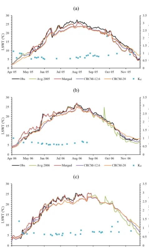
Figure 4 compares the results of different LSWT FLake simulations with observations at the NDBC station. LSWT observations had maximum values of 27.53, 26.48, and 25.46◦C in August during 2005, 2006 and 2007, respec-tively. The minimum values of 2.71, 7.3, and 3.42◦_{C were}

observed in December 2005, and April in 2006 and 2007, re-spectively. The average LSWT observations in 2005, 2006, and 2007 had values of 18.45, 17.12, and 17.75◦C, respec-tively. Four different simulation schemes were made which were then compared to the observed LSWT. The simulated LSWT values in Fig. 4 were produced by first applying Kd=0.2 m−1 from Martynov et al. (2012) using both the real lake depth at the station (12.6 m: CRCM-12.6) and also a tile depth corresponding to the station in their study (20 m: CRCM-20). Then, simulations using the yearly average CC-derivedKdfor each year of study were plotted (Avg). TheKd values derived from the monthly average of each year were used to simulate the surface water temperature and produce a merged LSWT product (Merged). Both Avg and Merged simulations used the real lake depth at the NDBC station (12.6 m).

Table 2.CC-derived average values ofKdfor each month (2005–2007). The values correspond to the time of year when water LSWT observations, as well as the CC derivedKdvalues, are available.

Year April May June July August September October November Average

2005 – 0.69 0.62 0.63 0.79 1.07 0.92 0.97 0.81 2006 0.82 0.70 0.62 0.65 0.77 – – – 0.71 2007 0.86 0.72 0.64 0.65 0.76 – – – 0.73

Figure 4. Daily LSWT simulation results in 2005(a), 2006 (b), 2007(c). Avg. simulation is the CoastColour-derived average value for Kd during selected months of each year (0.81, 0.71, and 0.73 m−1, respectively). Merged simulation is based on merging simulation results for monthly average values ofKd. CRCM-12.6 and CRCM-20 used a constant value ofKd(0.2 m−1) with depth values of 12.6 and 20 m, respectively. The corresponding observa-tions for LSWT are also plotted. Missing lines indicate no data.

Table 3.Simulated LSWT compared to in situ observations (2005– 2007). Period corresponds to the time of year when LSWT andKd values were available.

Period Kd RMSE MBE Ia

Avg2005 1.69 −0.86 0.87 2005 Merged 1.76 −0.95 0.86 May–Nov CRCM-12.6 1.88 −1.52 0.85 CRCM-20 2.12 −1.54 0.83

Avg2006 1.40 0.59 0.89 2006 Merged 1.42 0.54 0.89 Apr–Aug CRCM-12.6 1.50 −0.98 0.89 CRCM-20 1.47 −1.09 0.89

Avg2007 1.37 0.62 0.90 2007 Merged 1.35 0.57 0.91 Apr–Aug CRCM-12.6 1.78 −1.08 0.86 CRCM-20 1.80 −1.35 0.87

MBEMerged= −0.75◦C; fall: MBEAvg= −1.82◦C, MBEMerged= −1.99◦C; see Fig. 5 for seasonal-based performance of simulations). CRCM-12.6 and CRCM-20 were reproducing a colder LSWT on average with max-imum under-prediction in July–August (for 2005–2007: −2.93◦C<MBEJuly-August <−0.99◦C). Simulation with a larger depth (CRCM-20) tended to gain (lose) heat more slowly in spring (fall), compared to all other simulations.

Figure 5.Modeled (yaxis) versus observed (xaxis) LSWT for yearly average, merged, CRCM-12.6, and CRCM-20 simulations during the ice-free seasons in 2005–2007. A linear fit (dashed line) and its coefficients are shown on the plot. The statistics related to the regression of parameters, and a 1:1 relationship (solid line) are also shown. The average LSWT values of Obs, Avg, Merged CRCM-12.6, and CRCM-20 simulations are 18.64, 18.56, 18.50, 17.38, and 17.27◦C, respectively.

Therefore, a yearly-average Kdcan be potentially closer to the actual value of Kd. For this reason, the merged results cannot always perform better than average simulations.

Figure 5 illustrates the scatterplots of simulated LSWT for all four different runs including 3 years of data (2005– 2007), in comparison with the corresponding in situ obser-vations. All simulated results were in a high agreement with in situ measurements. Figure 5a and b show that the result-ing LSWT from yearly average (Avg) and monthly average (Merged)Kdwere not significantly different, whereas simu-lations with yearly averageKdreproduced LSWT with im-proved RMSE and MBE values compared to monthly av-erages (Avg: RMSE=1.54◦C, MBE= −0.08◦C; Merged: RMSE=1.57◦C, MBE= −0.14◦C). It is possible that the actual Kd value is best represented by the yearly average value. Therefore, using a constant annual open water sea-son value for Kd could be potentially sufficient to simu-late LSWT in 1-D lake models with relatively high accuracy (the range of Kd variations that brings the most sensitivity for the modeling is discussed in Sect. 3.2.2). Both CRCM

simulations (Fig. 5c: depths of 12.6 and Fig. 5d: depth of 20 m) under-predicted LSWT (for LSWT values larger than ca. 7◦C), with MBE values of −1.26 and −1.37◦C, re-spectively. The under-prediction of these model runs was stronger, particularly for LSWT above 12◦_{C, which can be}

explained by theKd value used. This is because, no mat-ter what depth is used in simulations (either actual or tile depth), both CRCM runs have larger MBE compared to Avg and Merged simulations. However, the CRCM-20 simula-tion tended to produce the coldest LSWT (the most under-predicted; MBE= −1.37◦C). This is due to the lake depth value considered for the model run, which corresponds to the tile depth as opposed to the other simulations that were based on using the actual depth at the station.

(Avg: RMSE=1.54◦C, MBE= −0.08◦C; CRCM-12.6: RMSE=1.76◦_{C, MBE= −1.26}◦_{C). Under-prediction of}

LSWT decreased when the yearly-average CC-derived Kd values were used, rather than a generic constant value (0.2 m−1). Heiskanen et al. (2015) suggested that the effect of Kdseasonal variations on LSWT simulations are not signifi-cant for lakes withKdvalues higher than 0.5 m−1(e.g., Lake Erie). Therefore, in the absence of reliable values of the tem-poral evolution ofKd, a lake-specific, time-independent, and constant value ofKdcan be used in 1-D lake models when theKdvalues are higher than 0.5 m−1.

Martynov et al. (2012) concluded that applying a more realistic lake depth parameterization improves the FLake model performance. Using the realistic lake depth (12.6 m) at the NDBC station slightly improves the model per-formance in reproducing LSWT compared to a sim-ulation employing the corresponding tile depth (20 m) (CRCM-12.6: RMSE=1.76◦_{C, MBE= −1.26}◦_C;

CRCM-20: RMSE=1.88◦C, MBE= −1.37◦C) (Fig. 5c, d).

3.2.2 Sensitivity of FLake toKdvariations

The sensitivity of FLake to different values ofKdto repro-duce LSWT, MWCT, LBWT, MLD, isotherm, and ice phe-nology and thickness was investigated in this section for the year 2008. As indicated previously (Sect. 2.1), shortwave ir-radiance measurements were available in that year and long-wave irradiance was also measured from May to October 2008. Therefore, longwave irradiance for the other months of 2008 was modeled as described in Sect. 2.2 to fill the tem-poral gaps. Figure 6 presents simulation results for LSWT, MWCT, and LBWT using the real lake depth at the NDBC station, and the lowest, average, and highest values ofKd ob-served in the study period (minimumKd=0.58 m−1, aver-age Kd=0.90 m−1, maximumKd=3.54 m−1). The water temperature simulation from CRCM-12.6 (using Kd=0.2 and realistic depth at station) simulation was also plotted.

In the case of extreme clear water (CRCM-12.6), LSWT showed smoother variations during the open water season in 2008 as opposed to the darkest water simulation (max-imum, or Max) which displayed more abrupt LSWT vari-ations (Fig. 6). This is because solar radiation is absorbed more in waters with low clarity due to existing particles in water. It penetrates less deeply and warms up only the shal-low surface layer (which shows in shal-lower LBWT; see Fig. 6c) causing thinner mixing depth (Fig. 6d). The high tempera-ture of this shallow layer causes an increase in latent and sensible heat fluxes. Therefore, the shallow mixed layer ex-changes heat faster with the atmosphere, resulting in sud-den surface water temperature variations as opposed to clear waters. The fast heat exchange with atmosphere resulted in warmer LSWT during spring (start of heating season) and colder LSWT in fall for dark water as opposed to clear wa-ter. On average, the darkest water simulation (Max) resulted in 0.09◦C higher LSWT compared to the average (Avg)

sim-Figure 6.LSWT(a), MWCT(b), LBWT(c)and MLD(d) simula-tion results in 2008 for CRCM-12.6 (K_d=0.2 m−1) simulation and the lowest (Min,Kd=0.58 m−1), average (Avg,Kd=0.90 m−1), and highest (Max,Kd=3.54 m−1)Kdvalues are shown.

re-Figure 7. Isotherms in open water period 2008 for CRCM-12.6 (Kd=0.2 m−1) simulation and the lowest (Min,Kd=0.58 m−1), average (Avg,Kd=0.90 m−1), and highest (Max,Kd=3.54 m−1) Kdvalues are shown.

sults showed that FLake-simulated LSWT was not signifi-cantly sensitive to Kd values when this value varied in the range of our Min to Max Kd. However, the sensitivity in-creased rapidly forKdvalues less than our Min (0.58 m−1). This result supported the study of Rinke et al. (2010) that the thermal structure of lakes is particularly sensitive to changes in Kd when its value is below 0.5 m−1. More re-cently, Heiskanen et al. (2015) confirmed the critical thresh-old ofKd(ca. 0.5 m−1). They suggested that the response of 1-D lake models to Kdvariations is nonlinear. The models are much more sensitive if the water is estimated to be too clear. Heiskanen et al. (2015) recommended to use a value of Kdthat is too high rather than too low in lake simulations, if the clarity of lake is not known exactly.

The MWCT and LBWT in the darkest condition (Max) were less than for all other clear-water simulations. This is because the lower layers in dark waters accumulate less heat during the heating season as opposed to clear wa-ters, which results in less heat storage and lower water col-umn temperature in dark waters (Heiskanen et al., 2015; Potes et al., 2012). The MWCT decreased by 0.94◦C (in-creased by 0.63◦C) when maximum (minimum) Kd value was used instead of its average value during the study pe-riod. The MWCT increased by 2.25◦C when using a Kd value of 0.2 m−1rather than the average value. Changes in Kdvalue from its maximum (minimum) to its average value also caused a decrease (increase) of −0.67◦_{C (0.67}◦_{C) in}

the LBWT. The increase in LWBT was even larger when the Kd value of 0.2 m−1 was used instead of its average value (6.96◦C). Therefore,Kd variations had a larger impact on MWCT and LBWT than on LSWT, and the largest differ-ence was whenKdwas estimated to be extremely clear.

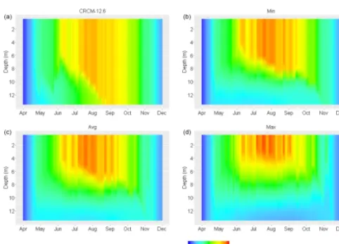
Figure 7 displays the simulated isotherms derived from us-ing differentKdvalues. It shows that the mixed layer in dark

waters was warmer in spring and summer and colder in fall. There are a number of factors determining the mixed-layer temperature in lakes, including the radiation fluxes (sensible heat, latent heat, and longwave radiation), and cooling effects from the water below. Persson and Jones (2008) concluded that for dark waters, the combination of these heating and cooling effects leads to a warmer epilimnion initially. The radiation is used to warm up a thinner layer in dark waters leading to higher (lower) temperatures in spring and sum-mer (fall). However, a lower temperature in the mixed layer is followed due to the gradual decrease in radiative forcing and increased effect of cooling from the layers below. Fig-ure 7 also supports observations by Persson and Jones (2008) and Heiskanen et al. (2015) that the depth of the thermo-cline layer is always deeper in clear waters due to the faster heat distribution between different underneath layers. The deepening of the thermocline layer in clear waters is faster compared to dark waters. The reason is related to heat trans-fer through convection, wind-induced mixing, and internal waves. The heat transfer in dark waters is slower due to the sharp density gradient between layers which forms an effec-tive barrier for the mixing to deepen the thermocline.

Figure 6d is focusing on the variations of the MLD in 2008, using different values ofKd(Min, Avg, and MaxKd, and CRCM-12.6) in simulations. All simulations showed two turnover (complete mixing) events, spring and fall. Full mix-ing in sprmix-ing was at the same time for all simulations; how-ever, fall full mixing occurred at different dates for each sim-ulation. Fall turnover in CRCM-12.6 was at the end of sum-mer (28 August), while the other three runs show that the fall turnover took place in late fall, before ice forms. Full mixing in the Min simulation was in early November (3 November), earlier than the Avg and Max simulations (21 November).

In the darkest water simulation (Max), the MLD was shallower than the other simulations (an average difference of 4.94 m in 2008 between two simulations of Max and CRCM-12.6, with extremeKd values). Clear waters have a deeper mixed layer when the solar radiation can penetrate further and distribute to a larger volume in the water col-umn. Also, due to the weak density gradient in clear wa-ters, wind-induced turbulent kinetic energy can destroy the density stratification to a deeper layer and form the mixed layer. This layer is shallower in dark waters, even with the same wind forcing. CRCM-12.6 produced a MLD of 3.47 m deeper compared to Avg simulation, whereas the Min (Max) simulations resulted in MLD 1.15 m (1.47 m) deeper (shal-lower) compared to the Avg simulation. Hence, clear water simulated deeper MLD; and the effect ofKd on the MLD was larger when theKdvalue was estimated to be too clear.

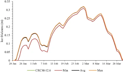
phenol-Figure 8. Ice thickness during 2008 for CRCM-12.6 (Kd= 0.2 m−1) simulation and the lowest (Min,Kd=0.58 m−1), aver-age (Avg,Kd=0.90 m−1), and highest (Max,Kd=3.54 m−1)Kd values are shown. CRCM-12.6 and Min (Avg and Max) simulations reproduce similar ice thicknesses, which explains the missing (hid-den) lines of CRCM-12.6 and Max simulations in the plot.

ogy as the Max simulation, whereas Min and CRCM-12.6 re-sulted in the similar up and freeze-up dates. The break-ups in CRCM-12.6 and Min simulations were on 23 March, 1 day earlier than Max and Avg simulations, and freeze-up occurred on 24 January, 2 days after Max and Avg simu-lations. CRCM-12.6 and Min simulations reproduced 1.28 and 1.27 cm thinner ice than Avg simulation in 2008, respec-tively. The darkest water (Max) reproduced 0.21 cm thicker ice in 2008 compared to the Avg simulation. The ice sheet formed later in clear waters (CRCM-12.6 and Min) and dis-appeared earlier compared to dark waters (Max and Avg), resulting in a shorter ice-cover duration (3 days) and hence thinner ice in clear-water simulations.

Lake morphological properties determine ice cover as well as climatic factors. Among morphological aspects, lake depth is the most important factor that can impact the ice cover by influencing the amount of heat storage in the wa-ter and hence the time needed for the lake to cool and ulti-mately freeze (Brown and Duguay, 2010). For a given depth and climatic condition, however, the amount of heat storage is determined by water clarity. Dark waters store more heat in a shallower layer. Therefore, the heat can be transferred faster to the atmosphere through the lake surface, resulting in an earlier freeze-up as mentioned in Heiskanen et al. (2015), who reported that freeze-up occurs earlier in darker waters. However, as shown by simulations with 12.6 m, ice phenol-ogy in the NDBC station was minimally affected byKdvalue in FLake. It must be noted that these results could not be ver-ified due to the lack of ice phenology observations. For a larger depth or in a different model, the impact ofKdvalues in ice onset should be investigated.

Figure 9.Spatial variation of satellite-derivedKdin Lake Erie, on 3 September 2011. Location of NDBC station is shown on the map as a solid dot.

3.3 Spatial and temporal variations inKd

As described in the previous section, variations in water clarity play an important role in defining lake heat budget and thermal stratification and thus is a significant param-eter for processes in the air–water interface. However, the long-term spatial and temporal trends of water clarity can-not be achieved through discontinuous conventional point-wise in situ sampling. These observations can be provided from satellite measurements. This section demonstrates the strength of satellite observations to detect the spatial and tem-poral variations ofKdin Lake Erie. Spatial variations ofKd derived from the CC algorithm are shown in Fig. 9 for a se-lected day (3 September 2011). This particular day of 2011 was selected as the lake experienced its largest algal bloom in its recorded history in that year, before the new recent record of 2015 (Michalak et al., 2013; NOAA, 2015). The bloom was expanding from the western basin into the central basin. Algal bloom is one of the factors affecting the water clarity of Lake Erie (NOAA, 2015). Other parameters include the con-centrations of suspended and dissolved matters in the lake. The western basin is the shallowest region of the lake, and therefore is the most vulnerable to sediment re-suspension that also results in reducing water clarity. The map shows that Lake Erie experienced different levels of clarity in var-ious locations, with an averageKdvalue of 0.90 m−1 (with standard deviation of 0.80 m−1, shown as 0.90±0.80 m−1 hereinafter) over the entire lake on this particular day. The NDBC station is also shown on the satellite-derived map as a reference (withKd=0.87 m−1on 3 September 2011).

Figure 10.Temporal and spatial variation of satellite-derivedKdin Lake Erie for different months of a year: May–August 2010. Location of the NDBC station is shown on the map as a solid dot.

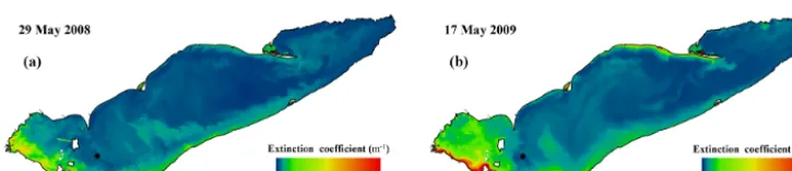
Figure 11.Temporal and spatial variation ofKdin Lake Erie during May of 2 consecutive years: 2008 and 2009. Location of the NDBC station is shown on the map as a solid dot.

of a spring algal bloom, and also wind-driven re-suspension of sediments. Kd at the NDBC station for these selected days varied between 0.68, 0.62, 0.66, and 0.85 m−1from the months of May to August 2010, respectively.

Two MERIS images with full coverage of Lake Erie were only available in the month of May for 2 selected consecutive years (2008 and 2009) to show the inter-annual changes in Kdvalue. Hence, the MERIS images of May 2008 and May 2009 were selected to show variations inKdbetween the two years. Although the images are for the same month of the year,Kdstill varied across the lake (Fig. 11). In the selected day of May 2008, a spatial average value of 0.77±0.49 m−1 was estimated for the entire lake, while on 17 May 2009 the spatial average value was 0.90±0.93 m−1. Comparing the estimated maps for the two years suggested that the spring bloom in 2009 was stronger than the one in 2008 for the west-ern basin. However, algal bloom in all basins of Lake Erie for the complete year of 2008 was recorded as the third-largest that the lake experienced before the occurrence of the break-ing record blooms in 2011 and 2015 (Michalak et al., 2013; NOAA, 2015). Kd values estimated for the NDBC station were 0.69 and 0.62 m−1_{on 29 May 2008 and 17 May 2009,} respectively.

Spatial variability ofKdin Lake Erie shows that the simu-lated thermal structure of the eastern basin would potentially differ significantly from the one simulated for the western

basin. The spatial variations of Kd have to be considered in Lake Erie simulations, specifically for the eastern basin, which hasKdvalues in the critical threshold range (less than 0.5 m−1). Therefore, in 3-D lake models, the spatial varia-tions inKdneed to be taken into account. As well as this, a lake-specific constant value cannot be used for simulating the thermal structure of the full lake. Finally, the temporal variations ofKddid not significantly change the simulation results for the NDBC station. However, this needs to be con-firmed for other locations of the lake, due to the importance of depth on the simulation results.

4 Summary and conclusion

Spatial and temporal variations ofKdin Lake Erie were de-rived from the globally available satellite-based CC product during open water seasons 2003–2012. The CC product was evaluated against SDD in situ measurements. CC-derivedKd values and modeled incoming radiation flux data, in addi-tion to complementary meteorological observaaddi-tions during the study period, were used to force the 1-D FLake model. The model was run for a selected site (NDBC buoy station) on Lake Erie, a large shallow temperate freshwater lake.

pre-vious study which assumed a constant Kdvalue due to the lack of data. Results clearly showed that applying satellite-derivedKdvalues improves FLake model simulations using a derived yearly average value as well as monthly averaged values of Kd. Although Kdvaries in time, a time-invariant (constant) annual value is sufficient for obtaining reliable estimates of lake surface water temperature (LSWT) with FLake for Lake Erie NDBC station. It was also shown that the model is very sensitive to variations inKdwhen the value is less than 0.5 m−1. This finding is in agreement with the study of Rinke et al. (2010) and the recent study of Heiska-nen et al. (2015) who determined that the impact of seasonal variations ofKdon the simulated thermal structure is small, for a lake with Kd values larger than 0.5 m−1. The studies suggested that the response of 1-D lake models toKd varia-tions is nonlinear. The models are much more sensitive if the water is estimated to be too clear. The results of our study showed that the sensitivity toKd variations was more pro-nounced in simulation results for mean water column tem-perature (MWCT), lake bottom water temtem-perature (LBWT), and mixed layer depth (MLD) compared to LSWT.

Results of this study have important implications for the lake modeling community, demonstrating that integrating satellite-derived lake-specificKdvalues can improve the per-formance of 1-D lake models compared to using a “generic” constantKd value. Although field measurements ofKd are not widely available, this study evaluated the strength of satellite observations and introduces them as a reliable data source to provide lake models with global estimates of Kd with high spatial and temporal resolutions. However, the weakness of this method is that the availability of satellite-derived Kd product can be limited due to cloud coverage or satellite overpass. Also, the in situ measurements are still required for validating satellite observations, because the in situ data collection remains the most accurate solution for water clarity measurement. The accuracy of the satellite-derivedKdproduct has to be verified for the water body of interest, especially for the ones with complex optical proper-ties. After validation, the on-demand globally available CC product can be simply used for the water body of interest, as a source to fill the gaps inKdin situ observations, and improve the performance of parameterization schemes and, as a re-sult, further improve the NWP and climate models. Although MERIS is no longer active, the Ocean and Land Colour In-strument (OLCI), to be operated on the ESA Sentinel-3 satel-lite (launched on 16 February 2016), will provide continu-ity of MERIS-like data. OLCI has MERIS heritages and im-proves upon it with an additional six spectral bands. There-fore, investigation of the Sentinel-3 potential to provide lake modeling community with the water clarity information is the next step of the current study. Also, the possible improve-ment in FLake output, when forcing the model with air hu-midity data collected directly at the station, can be examined in the future studies.

5 Data availability

The FLake model is available at http://www.flake.igb-berlin. de/. The shortwave irradiance was downloaded from SolarAnywhere®(https://www.solaranywhere.com), a prod-uct of SUNY model (Version 2.4). The shortwave and longwave irradiance in situ observations were provided by Ram Yerubandi in the National Water Research Institute (NWRI), Environment and Climate Change Canada (ECCC). The meteorological data (mean daily air temperature, wind speed, and water temperature measurements) were down-loaded from the website of the National Data Buoy Center (NDBC) of NOAA with free access (http://www.ndbc.noaa. gov/station_page.php?station=45005). Other meteorological data (air humidity and cloudiness) were purchased from the Ontario Climate Center (OCC), ECCC. CoastColour-derived extinction coefficient data were downloaded from the Coast-Colour website with free access (http://www.coastcolour.org/ products.html). The optical in situ data of Lake Erie was pro-vided by Caren Binding in ECCC.

Supplementary data are available at

doi:10.1594/PANGAEA.870520.

Author contributions. The presented research is the direct result of a collaboration with the listed co-authors. All materials used in the composition of the research article are the sole production of the primary investigator, listed as the first author. Claude R. Duguay and Homa Kheyrollah Pour supported this research through comments and advice related to the FLake model. The manuscript was edited for content and composition by the co-authors.

Competing interests. The authors declare that they have no conflict of interest.

Acknowledgements. The authors would like to thank Caren Binding (Environment and Climate Change Canada) for providing the optical in situ data of Lake Erie, Ram Yerubandi (Environment and Climate Change Canada) for providing the meteorological station data for Lake Erie, and Andrey Martynov for providing advice related to running the FLake model. Financial assistance was provided through a Discovery Grant from the Natural Sciences and Engineering Research Council of Canada (NSERC) to Claude Duguay. We also thank three anonymous reviewers for their valuable comments, which helped improve the paper.

Edited by: A. Weerts

Reviewed by: three anonymous referees

References

Arst, H., Erm, A., Herlevi, A., Kutser, T., Leppäranta, M., Reinart, A., and Virta, J.: Optical properties of boreal lake waters in Fin-land and Estonia, Boreal Environ. Res., 13, 133–158, 2008. Attila, J., Koponen, S., Kallio, K., Lindfors, A., Kaitala, S., and

Ylostalo, P.: MERIS Case II water processor comparison on coastal sites of the northern Baltic Sea, Remote Sens. Environ., 128, 138–149, 2013.

Binding, C. E. Jerome, J. H., Bukata, R. P., and Booty, W. G.: Trends in water clarity of the lower Great Lakes from remotely sensed aquatic color, J. Great Lakes Res., 33, 828–841, 2007.

Binding, C. E., Greenberg, T. A., Watson, S. B., Rastin, S., and Gould, J.: Long term water clarity changes in North America’s Great Lakes from multi-sensor satellite observations, Limnol. Oceanogr., 60, 1967–1995, 2015.

Bootsma, H. and Hecky, R.: A comparative introduction to the bi-ology and limnbi-ology of the African Great Lakes, J. Great Lakes Res., 29, 3–18, 2003.

Brown, L. C. and Duguay, C. R.: The response and role of ice cover in lake-climate interactions, Prog. Phys. Geog., 34, 671– 704, 2010.

Daher, S.: Lake Erie LAMP Status Report, 1-267, U.S. EPA and Environment Canada, 2000.

De Bruijn, E. I. F., Bosveld, F. C., and Van Der Plas, E. V.: An in-tercomparison study of ice thickness models in the Netherlands, Tellus A, 66, 21244–21255, 2014.

Duguay, C. R., Flato, G. M., Jeffries, M. O., Ménard, P., Morris, K., and Rouse, W. R.: Ice-cover variability on shallow lakes at high latitudes: Model simulations and observations, Hydrol. Process., 17, 3465–3483, 2003.

Eerola, K., Rontu, L., Kourzeneva, E., and Shcherbak, E.: A study on effects of lake temperature and ice cover in HIRLAM, Boreal Environ. Res., 15, 130–142, 2010.

Gordon, H. R.: Can the Lambert-Beer law be applied to the diffuse attenuation coefficient of ocean water?, Limonol. Oceanogr., 34, 1389–1409, 1989.

Gueymard, C., Perez, R., Schlemmer, J., Hemker, K., Kivalov, S., and Kankiewicz, A.: Satellite-to-Irradiance Modeling – A New Version of the SUNY Model, 42nd IEEE PV Specialists Confer-ence, New Orleans, LA, June 2015.

Heiskanen, J. J., Mammarella, I., Ojala, A., Stepanenko, V., Erkkilä, K.-M., Miettinen, H., Sandström, H., Eugster, W., Leppäranta, M., Järvinen, H., Vesala, T., and Nordbo, A.: Effects of water clarity on lake stratification and lake-atmosphere heat exchange, J. Geophys. Res.-Atmos., 120, 7412–7428, 2015.

Hinzman, L. D., Goering, D. J., and Kane, D. L.: A distributed ther-mal model for calculating soil temperature profiles and depth of thaw in permafrost regions, J. Geophys. Res., 103, 28975–28991, 1998.

Kheyrollah Pour, H., Duguay, C. R., Martynov, A., and Brown, L. C.: Simulation of surface temperature and ice cover of large northern lakes with 1-D models: A comparison with MODIS satellite data and in situ measurements, Tellus A, 64, 17614– 17633, 2012.

Kheyrollah Pour, H., Duguay, C., Solberg, R., and Rudjord, Ø.: Impact of satellite-based lake surface observations on the initial state of HIRLAM. Part I: evaluation of remotely-sensed lake sur-face water temperature observations, Tellus A, 66, 21534–21546, 2014a.

Kheyrollah Pour, H., Rontu, L., and Duguay, C.: Impact of satellite-based lake surface observations on the initial state of HIRLAM. Part II: Analysis of lake surface temperature and ice cover, Tel-lus A, 66, 21395–21413, 2014b.

Kleissl, J., Perez, R., Cebecauer, T., and Šúri, M.: Solar En-ergy Forecasting and Resource Assessment, Elsevier, MA, USA, 2013.

Koenings, J. P. and Edmundson, J. A.: Secchi disk and photometer estimates of light regimes in Alaskan lakes: Effects of yellow color and turbidity, Limnol. Oceanogr., 36, 91–105, 1991. Kourzeneva, E.: External data for lake parameterization in

Numer-ical Weather Prediction and climate modeling, Boreal Environ. Res., 15, 165–177, 2010.

Kourzeneva, E., Martin, E., Batrak, Y., and Moigne, P. Le: Climate data for parameterisation of lakes in Numerical Weather Predic-tion models, Tellus A, 64, 17226–17243, 2012a.

Kourzeneva, E., Asensio, H., Martin, E., and Faroux, S.: Global gridded dataset of lake coverage and lake depth for use in nu-merical weather prediction and climate modelling, Tellus A, 64, 15640–15654, 2012b.

Martynov, A., Sushama, L., and Laprise, R.: Simulation of temper-ate freezing lakes by one-dimensional lake models: Performance assessment for interactive coupling with regional climate mod-els, Boreal Environ. Res., 15, 143–164, 2010.

Martynov, A., Sushama, L., Laprise, R., Winger, K., and Dugas, B.: Interactive lakes in the Canadian Regional Climate Model, ver-sion 5: The role of lakes in the regional climate of North Amer-ica, Tellus A, 64, 16226–16248, 2012.

Maykut, G. A. and Church, P. E.: Radiation Climate of Barrow Alaska, 1962–66, J. Appl. Meteorol., 12, 620–628, 1973. Michalak, A. M., Anderson, E. J., Beletsky, D., Boland, S., Bosch,

N. S., Bridgeman, T. B., Chaffin, J. D., Cho, K., Confesor, R., Daloglu, I., DePinto, J. V., Evans, M. A., Fahnenstiel, G. L., He, L., Ho, J. C., Jenkins, L., Johengen, T. H., Kuo, K. C., LaPorte, E., Liu, X., McWilliams, M. R., Moore, M. R., Posselt, D. J., Richards, R. P., Scavia, D., Steiner, A. L., Verhamme, E., Wright, D. M., and Zagorski, M. A.: Record-setting algal bloom in Lake Erie caused by agricultural and meteorological trends consistent with expected future conditions, P. Natl. Acad. Sci. USA, 110, 6448–6452, 2013.

Mironov, D.: Parameterization of lakes in numerical weather predic-tion. Part 1: Description of a lake model. Offenbach: Consortium for Small-scale Modeling, Technical Report 11, 47 pp., 2008. Mironov, D., Heise, E., Kourzeneva, E., Ritter, B., Schneider, N.,

and Terzhevik, A.: Implementation of the lake parameterisa-tion scheme FLake into the numerical weather predicparameterisa-tion model COSMO, Boreal Environ. Res., 15, 218–230, 2010.

Mironov, D., Ritter, B., Schulz, J.-P., Buchhold, M., Lange, M., and Machulskaya, E.: Parameterisation of sea and lake ice in numer-ical weather prediction models of the German Weather Service, Tellus A, 64, 17330–17346, 2012.

Moore, T. S., Dowell, M. D., Bradt, S., and Ruiz-Verdu, A.: An op-tical water type framework for selecting and blending retrievals from bio-optical algorithms in lakes and coastal waters, Remote Sens. Environ., 143, 97–111, 2014.

Olmanson, L., Brezonik, P., and Bauer, M.: hyperspectral remote sensing to assess spatial distribution of water quality character-istics in large rivers: The Mississippi River and its tributaries in Minnesota, Remote Sens. Environ., 130, 254–265, 2013. Persson, I. and Jones, I.: The effect of water colour on lake

hydro-dynamics: A modelling study, Freshwater Biol., 53, 2345–2355, 2008.

Poole, H. H. and Atkins, W. R. G.: Photo-electric measurements of submarine illumination throughout the year, Mar. Biol., 16, 297– 394, 1929.

Potes, M., Costa, M. J., and Salgado, R.: Satellite remote sens-ing of water turbidity in Alqueva reservoir and implications on lake modelling, Hydrol. Earth Syst. Sci., 16, 1623–1633, doi:10.5194/hess-16-1623-2012, 2012.

Rinke, K., Yeates, P., and Rothhaupt, K. O.: A simulation study of the feedback of phytoplankton on thermal structure via light ex-tinction, Freshwater Biol., 55, 1674–1693, 2010.

Ruescas, A., Brockmann, C., Stelzer, K., Tilstone, G. H., and Beltrán-Abaunza, J. M.: DUE Coastcolour Final Report, version 1, Brockmann Consult, , 2014.

Samuelsson, P., Kourzeneva, E., and Mironov, D.: The impact of lakes on the European climate as simulated by a regional climate model, Boreal Environ. Res., 15, 113–129, 2010.

Thiery, W., Martynov, A., Darchambeau, F., Descy, J.-P., Plisnier, P.-D., Sushama, L., and van Lipzig, N. P. M.: Understanding the performance of the FLake model over two African Great Lakes, Geosci. Model Dev., 7, 317–337, doi:10.5194/gmd-7-317-2014, 2014.

Wilcox, S.: National Solar Radiation Database 1991–2010 Update: User’s Manual, National Renewable Energy Laboratory, 2012. Willmott, C. J.: On the validation of models, Phys. Geogr., 2, 184–

194, 1981.

Willmott, C. J. and Wicks, D. E.: An Empirical Method for the Spatial Interpolation of Monthly Precipitation within California, Phys. Geogr., 1, 59–73, 1980.

Willmott, C. J., Robeson, S. M., and Matsuura, K.: A refined index of model performance, Int. J. Climatol., 32, 2088–2094, 2012. Wu, G., De Leeuw, J., and Liu, Y.: Understanding Seasonal

Wa-ter Clarity Dynamics of Lake Dahuchi from In Situ and Remote Sensing Data, Water Resour. Manag., 23, 1849–1861, 2008. Zhao, D., Cai, Y., Jiang, H., Xu, D., Zhang, W., and An, S.:

Estima-tion of water clarity in Taihu Lake and surrounding rivers using Landsat imagery, Adv. Water Resour., 34, 165–173, 2011. Zolfaghari, K. and Duguay, C. R.: Estimation of Water Quality

Pa-rameters in Lake Erie from MERIS Using Linear Mixed Effect Models, Remote Sens., 8, 473, doi:10.3390/rs8060473, 2016. Zolfaghari, K., Duguay, C. R., and Kheyrollah Pour, H.: