COMPARATIVE ANALYSIS OF TIME DOMAIN AND
FREQUENCY DOMAIN BLIND AUDIO SOURCE
SEPARATION TECHNIQUES
Naveen Dubey
1, Rajesh Mehra
21,2
Department of Electronics and Communication
National Institute of Technical Teacher Training and Research, Chandigarh (India)
ABSTRACT
This paper introduced comparative analysis of blind audio source separation techniques in time domain, frequency domain. In time domain analysis modified convex divergence method and ICA decomposition techniques are considered and in frequency domain Inter-frequency Correlation with Microphone Diversity techniques are considered. To perform this analysis a critically determined system consists of three audio sources and three microphones are considered. Frequency domain analysis can be implemented for over determined mixture also, in that it extracts principle component to form a determined mixture. Simulations are performed on a closed room recording samples and convergence speed and complexity is compared. Result reflects that divergence based ICA overshadows the other competitors in terms of convergence speed and proved as a better audio source separation technique in blind scenario.
I. INTRODUCTION
The objective of Blind Audio Source Separation (BASS) is intended to separate multiple independent audio
sources from an ill-informed mixing environment [1]. The general mixing model can be formulated as follows
[2];
)
(
)
(
)
(
)
(
t
A
t
s
t
t
M
(1)For the sake of simplicity ideal mixing environment can be considered by ignoring the role of noise
components. The model for source separation mathematically formulated as;
)
(
)
(
)
(
ˆ
t
W
t
M
t
S
(2)Where:
„t is the sample index and mathematical operation is matrix convolution.
Most of the frequency domain blind source separation algorithms uses weight overlap and add method or STFT
(short time Fourier transform) method for finding the coefficient of an equivalent filter, so that independent
sources can be separated. Frequency domain approach needed long duration of recordings to make conclusion
[3]. Frequency domain source separation approaches encounter two major problems; First the frequency domain
ICA suffers with permutation ambiguity in order of output. To counter that a wise criteria considered in various
component of same signal in bin‟p+1‟ should also arrive in output „k‟. If this condition proves false, then
algorithm needs to apply since beginning and result considered as mixed.
Second problem is, there is no information about magnitude of every frequency bin. If we assume perfect
separation and ignore permutation ambiguity issue, the magnitude still needs to be scaled by a constant in each
frequency bin. To achieve that an addition filter needs to be applied at output, which further increases the
complexicity of frequency domain techniques? Principle of minimal distortion [4] is a typical cure of this
problem, which rectifies any probable need of additional filtering at the output of the unmixing ICA algorithms.
Frequency domain algorithms also encounters bad bin problem when mixing system is over-determined.
In time-domain techniques the convolution model derived into an instantaneous form by incorporating matrices
or data vectors and the convolutive process is simply transformed into a matrix multiplication technique.
Matrices are defined from available signal data captured by microphones and treated as observation space.
Generally a matrix is defined so that its rows contain the time-lagged copies of signals received from
microphones. The objective of time domain ICA decomposition is to find out subspace that corresponds to
separated signals [5]. The observation space can be decomposed completely or partially [6]. In complete
decomposition the original signals are represented as “n” independent subspaces covering the entire observation
space. In partial decomposition signals are considered as one dimensional subspace
In this work a comparative analysis has been performed over three algorithms, on frequency domain algorithm
Inter-frequency correlation with microphone diversity (ICMD) [7] and two time domain first one modified
convex divergence and second one is time domain subspace decomposition method. Rest of the paper organized
as follows; section II consist of two time domain algorithms, section III explains ICMD algorithm, simulation
results and comparative analysis is being performed in section IV. Finally, section V consists of final
conclusion.
II. TIME DOMAIN ALGORITHMS
NC-ICA is convex divergence based algorithm; it is modified version of existing convex divergence ICA [8].
This algorithm is intended to determine estimate the unmixing weight matrix by introducing divergence based
unsupervised learning mechanism for weight updation. For ensuring non-Gaussianity positive kurtosis value
fixed as stopping criterion of algorithm. The modified divergence equation is as follows;
f
p
x
y
f
p
x
p
y
f
p
x
y
p
x
p
y
dxdy
y
x
D
NC(
,
,
)
{
(
(
,
))
(
1
)
(
(
)
(
))
(
(
,
)
(
1
)
(
)
(
))}
1 24 2
))
,
(
(
)
,
(
2
1
2
1
1
{
y
x
p
y
x
p
1 24 3
)
(
)
(
(
)
(
)
(
2
1
2
1
)
1
(
y
p
x
p
y
p
x
p
( ) ( ) 1 1 ) , ( 1 2 1 2 1 { 1 2 2 22 p x y p x p y
dxdy
y
p
x
p
y
x
p
(
)
(
)]
}}
1
1
)
,
(
1
[
1 2
1
2
α is convexity parameter
p(x,y) and p(y,x) are joint probability and p(x)
and p(y) are marginal probabilities.
In this algorithm first data needs to pre-processed by centring and whitening, then input data matrix applied into
algorithm for weight updation, Scaled natural gradient [9] learning method is adopted
) ( ) ( )
( ) ( )
( ) ( ) ( ) 1
(
(
,
,
)
tT tt t NC t t t t
W
W
W
W
D
d
c
W
W
(4)
Once algorithms stops after fulfilling the stopping criteria. Weight needs to normalise and centre removal
performed. And obtained estimated weight matrix applied as per equation (2) for estimation of source signals.
Second time domain algorithm is complete ICA decomposition of observation space. In this algorithms first, it
is assumed that M samples of simultaneously recorded from array of microphones are yi(n) y2(n). . . .. . ym(n).
And a matrix is created by delaying each recorded sample by l. Matrix Y is created
„y1[l]. . . . .. . . y1[M] „y1[l-1] . . . . .. . . y1[M-1]
. .
. .
Y= „y1[1] . . . y1[M-l+1]
„y2[l] . . . . ... y2[M]
. .
. .
„yn[1] . . ... . .. .. yn[M-l+1]
Figure 1 Decomposition Matrix
The ICA technique for separating audio sources from mixed signal can be classified on the foundation of
whether; they are performing complete or partial decomposition of available observation data space.
Apply above mentioned ICA algorithm to determine independent components. After determine the independent
clustering technique is applied to evaluate a cluster on the basis of similarity criterion. Once respective cluster is
formed reconstruction process is applied to determine independent sources.
III. FREQUENCY DOMAIN APPROACH
In frequency domain source separation technique author used ICMD techniques. In this method assuming the P
number of unknown sources, at each frequency only P microphones are fed to ICA algorithm to form output. By
this technique, we uses cascaded ICA initialization technique to check output permutation ambiguity.
Similar to all frequency domain algorithms, the input from all recording microphones are first needs to
transform from time domain to frequency domain using short time Fourier transform. Assuming that the number
[10] is “on observation based, the false alignment generally takes position where performance of separation is
poor”, In result of that, the output at one frequency bin could match with more than one bins output. Hence
mapping is not possible.
Let us consider Rxy(n-1, n) as a normalized cross-correlation sample matrix of the amplitudes of unmixing
signals in consecutive bins. Let‟s assume the vector of output signals
Xn(t)= [Xn(1,t). . . .Xn(P,t) ]T [5]
Where, Xn(P,t) is the pth output in the bin „n‟ at the sample time „t‟. Now the standard deviation of Xn(t) can be
estimated over time period „T‟. The normalized signal can be written as;
u
n(
t
)
x
n(
t
)
/
ˆ
x
,
n
(
p
)
[6]When the resulting output signal in both bins are obtained well separated and the same permutation holds in
both the cases , then cross-correlation will diagonally dominant. If there is permutation changes occur at output
then process needs to repeat again. All corresponding bins are detected and combine as per microphone diversity
and separated sources are obtained.
IV. SIMULATIONS AND RESULT DISCUSSIONS
To evaluate and compare performance of techniques discussed in prior section; three audio sources have been
taken, there were one male voice sample, one female voice sample and one recording of musical instrument. For
the sake of uniformity 20000 sample are taken of each audio source signal shown in figure 2. Mixing
environment is created by matrix convolution of source signals with a randomly generated matrix. Mixed
sources are shown in figure. 3
0 0.2 0.4 0.6 0.8 1 1.2 1.4 1.6 1.8 2 x 10⁴ -0.2
-0.15 -0.1 -0.05 0 0.05 0.1
0.15 s ourc e1
0 0.2 0.4 0.6 0.8 1 1.2 1.4 1.6 1.8 2 x 10⁴
-0.8 -0.6 -0.4 -0.2 0 0.2 0.4 0.6 0.8
1 s ourc e2
0 0.2 0.4 0.6 0.8 1 1.2 1.4 1.6 1.8 2 x 10⁴
-0.4 -0.3 -0.2 -0.1 0 0.1 0.2 0.3
0.4 s ourc e3
0 0.2 0.4 0.6 0.8 1 1.2 1.4 1.6 1.8 2 x 10⁴
-1.5 -1 -0.5 0 0.5 1 1.5 2
mix s ignal1
0 0.2 0.4 0.6 0.8 1 1.2 1.4 1.6 1.8 2 x 10⁴
-2 -1.5 -1 -0.5 0 0.5 1 1.5 2
mixsignal2
0 0.2 0.4 0.6 0.8 1 1.2 1.4 1.6 1.8 2 x 10⁴
-1.5 -1 -0.5 0 0.5 1 1.5
2 mix s ignal3
Figure 3 Mixed Signals 1,2,3
First modified convex divergence algorithm is applied where, convexity parameter are assumed as -1, results are
shown in figure 4. In this SIR values are 28.3, 31.2 , 33.1 dB respectively and execution time on AMD, 2.4 GHz
processor is 12 Seconds.
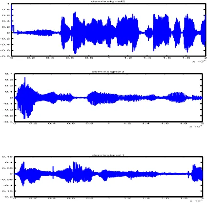
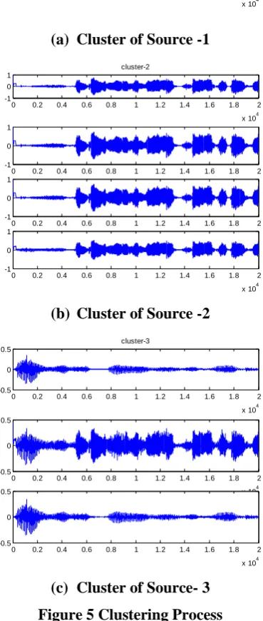
Second algorithm used is time domain subspace decomposition, in which k-mean clustering is used over
mixture of data and cluster results are shown in figure 5. In this techniques SIR values were 26.6, 29.2, 30.2 dB
respectively, and it takes execution time 16 second on same processor.
0 0.2 0.4 0.6 0.8 1 1.2 1.4 1.6 1.8 2 x 10⁴
-0.8 -0.6 -0.4 -0.2 0 0.2 0.4 0.6 0.8 1
demix s ignal2
0 0.2 0.4 0.6 0.8 1 1.2 1.4 1.6 1.8 2
x 104
-0.4 -0.3 -0.2 -0.1 0 0.1 0.2 0.3
0.4 demix s ignal3
0 0. 2 0. 4 0. 6 0. 8 1 1. 2 1. 4 1. 6 1. 8 2 x 10⁴
-0. 2 -0. 15 -0. 1 -0. 05 0 0. 05 0. 1 0. 15
demix s ignal1
0 0.2 0.4 0.6 0.8 1 1.2 1.4 1.6 1.8 2 x 10⁴ -0.2
0 0.2
cluster-1
0 0.2 0.4 0.6 0.8 1 1.2 1.4 1.6 1.8 2
x 104 -0.2
0 0.2
0 0.2 0.4 0.6 0.8 1 1.2 1.4 1.6 1.8 2
x 104 -0.5
0 0.5
(a)
Cluster of Source -1
0 0.2 0.4 0.6 0.8 1 1.2 1.4 1.6 1.8 2
x 104 -1
0 1
0 0.2 0.4 0.6 0.8 1 1.2 1.4 1.6 1.8 2
x 104 -1
0 1
0 0.2 0.4 0.6 0.8 1 1.2 1.4 1.6 1.8 2
x 104 -1
0 1
0 0.2 0.4 0.6 0.8 1 1.2 1.4 1.6 1.8 2
x 104 -1
0 1
cluster-2
(b)
Cluster of Source -2
0 0.2 0.4 0.6 0.8 1 1.2 1.4 1.6 1.8 2
x 104 -0.5
0 0.5
0 0.2 0.4 0.6 0.8 1 1.2 1.4 1.6 1.8 2
x 104 -0.5
0 0.5
0 0.2 0.4 0.6 0.8 1 1.2 1.4 1.6 1.8 2
x 104 -0.5
0 0.5
cluster-3
(c)
Cluster of Source- 3
Figure 5 Clustering Process
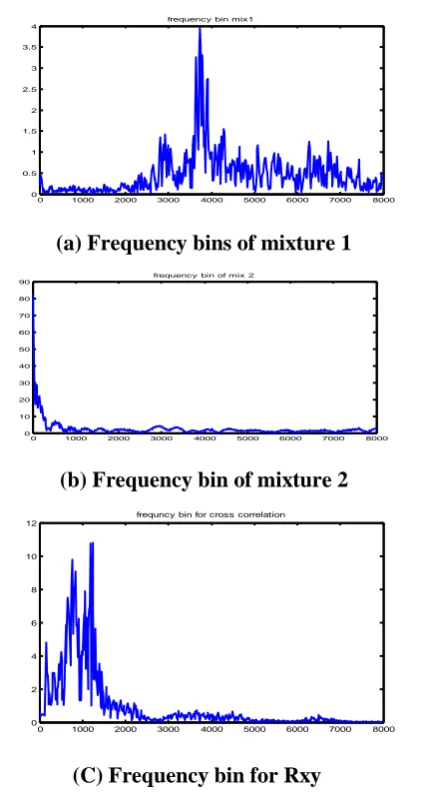
In third approach frequency domain techniques are used where various frequency bins are identified and
ICMD technique is applied. Some of the frequency bins are shown in figure 6 . Results reflects that
microphone diversity techniques suits well for real mixing environment, in artificial mixing environment
performance is inferior in comparison of time domain algorithms . It takes more time for separation, 22
0 1000 2000 3000 4000 5000 6000 7000 8000 0
0.5 1 1.5 2 2.5 3 3.5 4
frequency bin mix1
(a) Frequency bins of mixture 1
0 1000 2000 3000 4000 5000 6000 7000 8000 0
10 20 30 40 50 60 70 80 90
frequency bin of mix 2
(b) Frequency bin of mixture 2
0 1000 2000 3000 4000 5000 6000 7000 8000
0 2 4 6 8 10 12
frequncy bin for cross correlation
(C)
Frequency bin for Rxy
Figure 6 Frequency bins
Some more results were obtained but due to space limitation key results are shown Results reflects that , the
modified convex divergence based algorithm converges faster than other two competitor and also gives good
quality of separation. Here any straight comment could not be made on frequency domain algorithms as ICMD
is better suited for real experimental arrangements.
V. CONCLUSION
In this paper a comparative analysis being performed over two time domain algorithm and one frequency
domain algorithms. Results are evident that various source separation techniques provide better speed and
separation quality in case of audio source separation. The modified divergence based algorithms exhibits better
performance for specific value of convexity parameter. The clustering and decomposition techniques of
observation subspace also offers better performance. In this experiment the performance of frequency domain
algorithm was inferior somewhere but its not true always. ICMD could exhibit a quality performance in a real
REFERENCES
[1]. Naveen Dubey, Rajesh Mehra, “Blind Audio Source Separation: An unsupervised approach”, Int. Journal
of Electrical & Electronics Engg .Vol. 2, Spl. Issue 1 (2015) e-ISSN:1694-2310,pp.29-33
[2] Christopher Osterwise, Steven L. Grant, “On Over-Determined Frequency Domanin BSS”, IEEE/ACM
Trans. On Audio, Speech and Language Proc. Vol. 22, No. 5, pp. 956-966. May 2014
[3] Zbynek Koldovsky, Petr Tichavsky, “Time-Domain Blind Separation of Audio Sources on the Basis of a
complete ICA Decomposition of an Observation Space”, IEEE Trans. On Audio, Speech and Language
Proc. Vol. 19, No. 2 , pp. 406-416, Feb 2011
[4] K. Matsuoka, “Minimal distortion principle for blind source separation”, in proc. 41st SICE Annual conf,
Aug 5-7, 2002, Vol. 4, pp. 2138-2143.
[5] E. Vincent , R. Gribonval and M. D Plomby, “Oracle estimation for benchmarking of source separation
algorithms‟” Signal Processing , Vol.87, No.8, pp. 1933-1950, Nov, 2007.
[6]. S. C Douglas, H. Sawada and S. Makino, “Natural gradient multichannel blind deconvolution and
equalization using natural gradient,” in processing IEEE workshop signal processing Adv. In wireless
communication, paris, France, Apr. 1997 pp 101-104
[7] H. Sawada, R. Mukai, S. Araki and S. Makino, “Grouping separated frequency components by estimating
propagation model parameters in frequency domain blind source separation,” IEEE Trans. Audio, Speech
and Lang. Processing, Vol. 15, No.5, pp. 1592-1604, Jul 2007
[8] H. Bousbia-Salah, A. Belouchrani , and K abed-Meriam, “Jaccobi-like algorithm for blind signal
separation of convolutive mixtures”, IEE Electronics Letter, Vol. 37, No. 16, pp. 1049-1050, Aug. 2001
[9] Y. Chen, “Blind separation using convex function,”IEEE Trans. Signal Process., Vol. 53, No. 6, pp. 2027–
2035, Jun. 2005.
[10] Jen-Tzung Chien and Hsin-Lung Hsieh, “Convex Divergence ICA for Blind Source Separation”, IEEE
Trans. Audio, Speech, and Language Processing, Vol. 20, No. 01, pp. 302-314, January, 2012.
Naveen Dubey is currently associated with Electronics and Communication Engineering Department of RKG
Institute of Technology for Women, Ghaziabad, India since 2008. He is ME-Scholar atNational Institute of Technical Teachers‟ Training & Research, Chandigarh, India and received Bachelor of Technology from UP
Technical University, Lucknow, India in 2008. Received best performer award in creativity and innovation from
IIT-Delhi. He guided 20 UG projects and presented 2 projects in Department of Science and Technology,
Government of India. He published and presented more than 10 papers in International conferences and
journals. His research areas are Digital Signal Processing, Neural Networks and EM Fields. His research project
includes Blind audio source separation.
Dr. Rajesh Mehra: Dr. Mehra is currently associated with Electronics and Communication Engineering Department of National Institute of Technical Teachers‟ Training & Research, Chandigarh, India since 1996. He
has received his Doctor of Philosophy in Engineering and Technology from Panjab University, Chandigarh,
India in 2015. Dr. Mehra received his Master of Engineering from Panjab Univeristy, Chandigarh, India in 2008
and Bachelor of Technology from NIT, Jalandhar, India in 1994. Dr. Mehra has 20 years of academic and
industry experience. He has more than 250 papers in his credit which are published in refereed International
Journals and Conferences. Dr. Mehra has 55 ME thesis in his credit. He has also authored one book on PLC &
SCADA. His research areas are Advanced Digital Signal Processing, VLSI Design, FPGA System Design,