University of Pennsylvania
ScholarlyCommons
Publicly Accessible Penn Dissertations
2017
Essays On Dynamic Incentive Design
Mustafa Dogan
University of Pennsylvania, [email protected]
Follow this and additional works at:
https://repository.upenn.edu/edissertations
Part of the
Economics Commons
This paper is posted at ScholarlyCommons.https://repository.upenn.edu/edissertations/2259
For more information, please [email protected].
Recommended Citation
Dogan, Mustafa, "Essays On Dynamic Incentive Design" (2017).Publicly Accessible Penn Dissertations. 2259.
Essays On Dynamic Incentive Design
Abstract
This dissertation consists of three essays that examine incentive problems within various dynamic environments. In Chapter 1, I study the optimal design of a dynamic regulatory system that encourages regulated agents to monitor their activities and voluntarily report their violations. Self-monitoring is a private and costly process, and comprises the core of the incentive problem. There are no monetary transfers. Instead, the regulator (she) uses future regulatory behavior for incentive provision. When the regulator has full commitment power, she can induce costly self-monitoring and revelation of ``bad news'' in the initial phase of the optimal policy. During this phase, the agent is promised a higher continuation utility (in the form of future regulatory approval) each time he discloses ``bad news''. If the regulator internalizes self-monitoring costs, the agent is either blacklisted or whitelisted in the long run. When she does not internalize these costs,
blacklisting is replaced by a temporary probation state, and whitelisting becomes the unique long run outcome. This result suggests that whitelisting, which may appear to be a form of regulatory capture, may instead be a consequence of optimal policy.
In Chapter 2, I study the dynamic pricing problem of a durable good monopolist with commitment power, when a new version of the good is expected at some point in the future. The new version of the good is superior to the existing one, bringing a higher flow utility. The buyers are heterogeneous in terms of their valuations and strategically time their purchases. When the arrival is a stationary stochastic process, the corresponding optimal price path is shown to be constant for both versions of the good, hence there is no delay on purchases and time is not used to discriminate over buyers, which is in line with the literature. However, if the arrival of the new version occurs at a commonly known deterministic date, then the price path may decrease over time, resulting in delayed purchases. For both arrival processes, posted prices is a sub-optimal selling mechanism. The sub-optimal one involves bundling of both versions of the good and selling them only together, which can easily be implemented by selling the initial version of the good with a replacement guarantee.
Finally, Chapter 3 examines the question under what conditions can automation be less desirable compared to human labor. We study a firm that has to decide between a human-human team and a human-machine team for production. The effort choice of a human employee is not observed by the manager, therefore the incentives need to be properly aligned. We argue that, despite the desirable benefits resulting from the partial substitution of labor with automated machines such as less costly machine input and reduced scope of moral hazard, the teams with only human employees can, under some conditions, be more preferred over the human-machine teams. This stems from the fact that, in all-human teams, the principal, through the selection of incentive scheme, can control the interaction among the agents and get benefit from the mutual monitoring capacity between them. The automation, however, eliminates this interaction and shuts down a channel that can potentially help to mitigate the overall agency problem.
Degree Type
Dissertation
Degree Name
Graduate Group
Economics
First Advisor
George J. Mailath
Subject Categories
ESSAYS ON DYNAMIC INCENTIVE DESIGN Mustafa Dogan
A DISSERTATION in
Economics
Presented to the Faculties of the University of Pennsylvania in
Partial Fulfillment of the Requirements for the Degree of Doctor of Philosophy
2017
Supervisor of Dissertation
George J. Mailath, Professor of Economics
Graduate Group Chairperson
Jesus Fernandez-Villaverde, Professor of Economics
Dissertation Committee
George J. Mailath, Professor of Economics Steven Matthews, Professor of Economics
ESSAYS ON DYNAMIC INCENTIVE DESIGN
c
COPYRIGHT
2017
ACKNOWLEDGEMENTS
I am extremely thankful to my advisor, Professor George Mailath, for his guidance and encouragement throughout my doctoral studies. I have benefited deeply from his intellect along the years that I spent at Penn. He is, and will always be a reference of academic perfection and diligence to me.
I also thank the other members of my dissertation committee, Steven Mathews, and Mallesh Pai, for their support. I am thankful to my co-author Pinar Yildirim. My research has also benefited from discussions with Aislinn Bohren, David Dillenberger, Ju Hu, Nicholas Janetos, Joonbae Lee, SangMok Lee, Andrew Postlewaite, Francisco Silva, Rakesh Vohra, Yuichi Yamamoto.
Kelly Quinn deserves a special thank for her constant willingness to help.
I am indebted to Ismail Benli, Ihsan Dogan, Selman Erol, Salih Ozaslan, Metin Uyanik, and especially Ramazan Bora for sincere friendship.
ABSTRACT
ESSAYS ON DYNAMIC INCENTIVE DESIGN
Mustafa Dogan
George J. Mailath
This dissertation consists of three essays that examine incentive problems within various dynamic environments. In Chapter 1, I study the optimal design of a dynamic regulatory system that encourages regulated agents to monitor their activities and voluntarily report their violations. Self-monitoring is a private and costly process, and comprises the core of the incentive problem. There are no monetary transfers. Instead, the regulator (she) uses future regulatory behavior for incentive provision. When the regulator has full commitment power, she can induce costly self-monitoring and revelation of “bad news” in the initial phase of the optimal policy. During this phase, the agent is promised a higher continuation utility (in the form of future regulatory approval) each time he discloses “bad news”. If the regulator internalizes self-monitoring costs, the agent is either blacklisted or whitelisted in the long run. When she does not internalize these costs, blacklisting is replaced by a temporary probation state, and whitelisting becomes the unique long run outcome. This result suggests that whitelisting, which may appear to be a form of regulatory capture, may instead be a consequence of optimal policy.
known deterministic date, then the price path may decrease over time, resulting in delayed purchases. For both arrival processes, posted prices is a sub-optimal selling mechanism. The optimal one involves bundling of both versions of the good and selling them only together, which can easily be implemented by selling the initial version of the good with a replacement guarantee.
TABLE OF CONTENTS
ACKNOWLEDGEMENTS . . . iv
ABSTRACT . . . v
LIST OF TABLES . . . xi
LIST OF ILLUSTRATIONS . . . xii
CHAPTER 1 : Dynamic Incentives for Self-Monitoring . . . 1
1.1 Introduction . . . 1
1.1.1 Literature Review . . . 6
1.2 Model . . . 9
1.2.1 Actions and Preferences . . . 13
1.2.2 An Alternative Interpretation . . . 14
1.2.3 Policy . . . 15
1.2.4 Stationary Representation . . . 17
1.2.5 Principal’s ProblemP . . . 18
1.3 Case 1: Principal Internalizes Cost . . . 19
1.3.1 Observable Information Acquisition . . . 19
1.3.2 Moral Hazard and The Optimal Policy . . . 23
1.3.3 Conditional Representation . . . 24
1.3.4 The problemPD . . . 27
1.3.5 The problemPN . . . 30
1.3.6 The problemP0. . . 32
1.4 Case 2: Principal Does Not Internalize Cost . . . 40
1.4.1 Observable Information Acquisition . . . 41
1.5 Limited Commitment . . . 50
1.6 Concluding Remarks . . . 53
CHAPTER 2 : Product Upgrades and Posted Prices . . . 54
2.1 Introduction . . . 54
2.1.1 Literature Review . . . 57
2.2 Model . . . 58
2.2.1 Stochastic Arrival . . . 60
2.2.2 Deterministic Arrival . . . 61
2.3 Optimal Posted Prices: Stochastic Arrival . . . 62
2.3.1 Benchmark I: Canonical Durable Good Monopoly . . . 62
2.3.2 Benchmark II: Product Upgrade without Anonymous Prices . . . 65
2.3.3 Sales With Posted Prices: Anonymity . . . 67
2.4 Deterministic Arrival . . . 74
2.5 Conclusion . . . 79
CHAPTER 3 : Man vs. Machine: When is automation inferior to human labor? . 81 3.1 Introduction . . . 81
3.2 Literature Review . . . 84
3.3 Model . . . 86
3.3.1 No-Automation Regime . . . 86
3.3.2 Automation Regime: . . . 88
3.4 Optimal Incentive Contract . . . 88
3.4.1 Optimal Incentive Scheme Under Automation . . . 89
3.4.2 Optimal Incentive Scheme Under No-Automation . . . 90
3.4.3 Static Environment . . . 92
3.4.4 Dynamic Environment . . . 93
3.4.5 Collusion and Renegotiation-proofness . . . 102
3.4.7 Human teams survive under costless automation . . . 106
3.5 Extensions . . . 108
3.5.1 Heterogeneous Effort Decision . . . 109
3.5.2 First Best Benchmark . . . 110
3.5.3 Human-Machine Team . . . 111
3.5.4 Human-Human Team . . . 112
3.6 Conclusions . . . 116
APPENDIX . . . 120
CHAPTER A : Appendix to Chapter 1 . . . 120
A.1 Proof of Lemma 1.1 . . . 120
A.2 Proof of Lemma 1.2 . . . 121
A.3 Proof of Lemma 1.3 . . . 122
A.4 Proof of Lemma 1.4 . . . 124
A.5 Proof of Proposition 1.1 . . . 125
A.6 Proof of Lemma 1.5 . . . 127
A.7 Proof of Proposition 1.2 . . . 128
A.8 Proof of Lemma 1.6 . . . 130
CHAPTER B : Appendix to Chapter 2 . . . 131
B.1 Proof of Lemma 2.1 . . . 131
B.2 Proof of Lemma 2.4 . . . 132
B.3 Proof of Proposition 2.1 . . . 136
B.4 Proof of Lemma 2.5 . . . 138
B.5 Proof of Lemma 2.6 . . . 139
B.6 Proof of Proposition 2.2 . . . 140
CHAPTER C : Appendix to Chapter 3 . . . 147
C.2 Proof of Lemma 3.2 . . . 148
C.3 Proof of Lemma 3.3 . . . 149
C.4 Proof of Proposition 3.4 . . . 156
C.5 Proof of Lemma 3.1 . . . 156
C.6 Proof of Proposition 3.5 . . . 161
C.7 Proof of Lemma 3.4 . . . 162
C.8 Proof of Proposition 3.6 . . . 164
LIST OF TABLES
TABLE 1.1 : Alternative Interpretation . . . 15
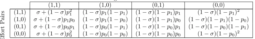
TABLE 3.1 : Joint Distribution of Signals . . . 87
LIST OF ILLUSTRATIONS
FIGURE 1.1 : The Stage Game . . . 14
FIGURE 1.2 : Value FunctionV∗. . . 22
FIGURE 1.3 : Representing Conditional Problem . . . 25
FIGURE 1.4 : Optimal Delegation Decisions in Case 1 . . . 35
FIGURE 1.5 : Value FunctionsVN, and VD . . . 38
FIGURE 1.6 : Value Function ˜V∗. . . 44
FIGURE 1.7 : Optimal Delegation Decisions in Case 2 . . . 46
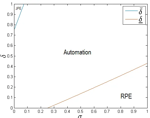
FIGURE 3.1 : Optimal Regime and Incentive Scheme . . . 106
FIGURE 3.2 : Optimal Regime, Costless Automation . . . 107
Chapter 1
Dynamic Incentives for Self-Monitoring
1.1
Introduction
The U.S. Environmental Protection Agency has an auditing policy that encourages compa-nies to monitor their ongoing and planned activities that may fall within its authority, and to voluntarily report their violations.1 This is an example of the framework that I explore in this paper. I am interested in understanding the behavior of regulators in environments where the regulated activity may result in bad outcomes and where there is significant un-certainty. Agents have an advantage in acquiring information about these activities because they have lower costs of monitoring. The regulator, in an efficient regulatory regime, would like to use agents’ self-monitoring. I study how regulators can induce economic agents to acquire and disclose costly information about the negative consequences of their activities through the use of future regulatory behavior without resorting to monetary transfers.
I show that, when the regulator has full commitment power, the optimal policy can induce self-monitoring only in an initial phase, which endures over a stochastic number of periods. When it ends, a terminal phase of the policy is initiated and self-monitoring stops.
1The auditing policy is defined in Environmental Protection Agency (11 April 2000), titled “Incentives
The outcome in this terminal phase is history-dependent and involves either blacklisting the agent or whitelisting him. When the regulator does not internalize self-monitoring costs, blacklisting is replaced by a temporary probation state. The unique long-run outcome is whitelisting in this case. This result suggests that whitelisting, which may appear to be a form of regulatory capture, may instead be a consequence of optimal policy. I also analyze the case in which the regulator’s commitment power is limited so that she cannot commit to policies with negative continuation values. In this case, if the expected cost of the social harm is larger than the economic benefits of the projects, then whitelisting never occurs in an optimal policy. Moreover, self-monitoring is sustained over the long term when the regulator does not internalize its costs.
In general, many enforcement authorities adopt self-monitoring practices for various regulatory purposes.2 A specific practice is the process of issuing licenses for activities with possible environmental consequences. A mining company, for example, in applying for a mining license, may be asked to submit an Environmental Impact Statement and sometimes other supplementary information that requires substantial and costly self-monitoring. The grant of the license empowers the company to operate and contributes to the aggregate economy. Yet, it may also cause some undesirable social consequences that the regulator needs to take into account.3 To make matters worse, these undesired outcomes oftentimes take a considerable amount of time to become apparent so that it is no more feasible to take ameliorating action.4 Therefore, investigating these potential harms prior to making a licensing decision is the only convenient policy for the regulator. And these investigations are delegated to the applicant company through the request of Environment Impact Statement.
Incentive divergence is the most prominent feature of the aforementioned settings. The agents prefer to avoid suspension of their activities and also generally prefer to avoid
mon-2
Securities and Exchange Commission, U.S. Department of Agriculture, U.S. Department of Defense, and Food and Drug Administration are examples.
3
For example, the mining area may have invisible connections to groundwater resources, in which case mining activities might lead to the production and the spread of hazardous material.
4
itoring due to its costs and the possibility of unfavorable signals that it might reveal. On the other hand, the regulators care about efficiency for which monitoring and suspending harm-producing activities are essential. Therefore, the regulator has a complicated policy problem that involves supervising the agents and at the same time incentivizing them to self-monitor.
To study the regulator’s problem, I construct a dynamic principal-agent model in which a stream of projects arrives over time, one for each period. The agent (he) wants to under-take the projects, but needs the approval of the regulator (she), who is the principal. The projects are ex-ante identical, yielding the same revenue for the agent. On the other hand, a project might either be harmless or it might result in social costs which would outweigh the value that the project generates. The agent can acquire information about whether the project has social costs by costly self-monitoring, but the efforts spent on self-monitoring are not directly observed by the principal. The principal has the objective of inducing socially preferable outcomes. Her preferences involve the economic benefits as well as the social costs resulting from these projects. Each period, the principal first decides whether or not to ask for self-monitoring, and then chooses whether to approve the project. There is no ex-post monitoring, and the realized harms are never observed. In many settings, the harms occur, or become evident, with a significant lag compared to the economic yields of the projects. To abstract from this reality, I analyze the case in which this lag goes to infinity.
There are no monetary transfers. In many situations, regulatory agencies are limited in their ability to use monetary transfers for various reasons. For example, in some industries there is a legal limitation on the size of the monetary fines that regulators can levy.5 As
a result, monetary transfers are too weak to induce proper behavior, and the regulator needs to use other tools for incentive provision. This paper focuses on the extreme case
5
of the regulators’ limited use of monetary transfers by ruling them out. In the absence of monetary transfers, the regulator provides incentives by linking her decisions over time.
The information structure governing the self-monitoring process takes the form of ver-ifiable “bad news” which are publicly observed. More precisely, there is a unique verver-ifiable signal perfectly revealing bad news and informing about the harm that will occur if the project is undertaken. In case the agent performs self-monitoring in a particular period, conditional on the project being harmful, the signal will be realized with some probability and will be publicly observed. If there is no news, then there are two possibilities from the principal’s perspective. First, the agent shirked and did not monitor. Second, the agent acquired information; however, no signal was realized since the project is more likely not to cause harm. There is no direct signal indicating good news. In most of the settings that fit into this paper, the only good news is the absence of bad news. In other words, certifiably disclosing good news is not possible. On the contrary, bad news, in general, pro-vides concrete evidence and detailed description of the harm that will occur if the project is undertaken. Conditional on this information structure, assuming that the signal is publicly observed is without loss of generality. As long as the agent prefers to monitor himself, he also prefers to disclose the signal in case it is realized. Otherwise, he could simply shirk in the first place and eliminate the cost of monitoring. The incentives that induce information acquisition automatically induces the disclosure contingent upon acquisition. Therefore, the signal remains public throughout the discussion in the paper, and hence self-disclosure exogenously occurs conditional on self-monitoring.
but the regulator promises more frequent approval in the future. If he does not disclose any signal, he is downgraded to a lower continuation utility. His current project has higher chances of approval, yet he will be given less frequent approvals in the future. The duration of this phase is stochastic; when it ends, the policy reaches a second phase in which there is no more self-monitoring. The transitional dynamics between the phases and the long-run outcome of the optimal policy depends on whether the principal internalizes the cost of self-monitoring.
If the principal internalizes the costs of self-monitoring, the acquired information is always used in the approval decision. The agent’s continuation utility eventually reaches either its minimum or maximum and remains constant. In this stage, the principal perma-nently rejects or permaperma-nently approves projects, that is, the agent is either blacklisted or whitelisted in the long run.6
When the principal does not internalize the self-monitoring costs, the content of the information is not always used in the current approval decision, in contrast to the previous case. There is a probation state, which replaces blacklisting, wherein the agent acquires information, but the project is rejected regardless of the outcome. The probation occurs when the agent’s continuation utility reaches its minimum in consequence of the agent not disclosing bad news frequent enough. After being initiated, this probationary state repeats until the agent discloses some bad news. Leaving the probation state today does not rule out the possibility of facing it again in the future. The agent’s continuation utility eventually reaches its maximum which still puts permanent approval into action, in the long run, the agent is always whitelisted.
The above-mentioned difference in the principal’s preferences alters the set of effec-tive inceneffec-tive devices she is willing to use. When she does not internalize its costs, self-monitoring can purely be used to punish the agent. It is possible for the principal to use
6
self-monitoring as punishment, because verifiability ensures that monitoring effort is taken. While the same channel was also feasible when the principal internalized the self-monitoring costs, she preferred not to punish this way because she cared about the cost.
In this model, whitelisting is an outcome of the optimal regulatory policy. Hence, I do not interpret it as a form of regulatory capture even though it shares some of its features. My paper, therefore, suggests that what has been described as regulatory capture in some cases may instead be an outcome of optimal regulatory policy.
Two situations give rise to inefficiencies in this framework. The first one occurs when the agent forgoes information acquisition, and the second one arises when the content of the information is not used efficiently. The first type only appears during the terminal phase of the optimal policy where there is no more self-monitoring. The second type, appears in the initial phase. Its occurrence triggers the terminal phase of the contract, when principal internalizes self-monitoring costs. Therefore, the inefficiencies are back-loaded in this case. However, when the principal does not internalize the self-monitoring costs, the second type of inefficiency occurs in a non-consecutive stochastic order, and its occurrence does not necessarily initiate the terminal phase. In this respect, efficiency will be lost and restored stochastically throughout the optimal policy.
I also study the situation in which the principal has limited commitment power, in that she cannot commit to a policy with a negative continuation value. The results change remarkably. If the expected cost of a project is higher than its economic benefit, the policy does not feature whitelisting. In this case, if the principal does not internalize self-monitoring costs, the policy never reaches a stable outcome and fluctuates over time.
1.1.1 Literature Review
of Becker (1968). By self-reporting a harmful act, the agent is granted a reduction in the sanctions he faces. In contrast to my model, the agent in their paper is initially endowed with the relevant information. Pfaff and Sanchirico (2000) introduce a more general framework in which the agency problem has two tiers: testing for noncompliance and fixing it.7 There is no information asymmetry to begin with, and the agent needs to exert effort to acquire relevant information. Most of the papers in this literature focus on characterizing the optimal incentive scheme in a static framework. My paper, however, studies the dynamics of a regulatory regime incorporating self-monitoring. In a contemporaneous work, Wang et al. (2016) also study a similar dynamic environment. The main distinction is that the harms are already known to agent and monetary transfers are allowed in their framework. They show that the optimal regime, in order to induce the agent to disclose harms, incorporates a cyclical structure alternating between rewarding self-disclosure and initiating inspections. Departing from theirs, my paper provides some explanation for practices such as blacklisting which arise from dynamic consequences.
In its use of non-monetary intertemporal incentives as a disciplining device, this paper relates to several different branches of literature. In mechanism design, Horner and Guo (2015) (HG) analyze a dynamic allocation problem in the absence of monetary transfers. The principal is interested in efficiency, which requires that the principal allocate the good only if the agent has a high valuation. The optimal mechanism follows a history-dependent rule which eventually converges to permanent allocation or permanent rejection of allo-cation. In the literature on relational contracts, Li et al. (2015) analyze the evolution of power inside organizations within the context of what they call a repeated trust game. The efficient equilibrium has a structure similar to that of HG, incorporating a bipolar long run outcome with permanent punishment and permanent rewards for the agent. Both of these papers assumes that the agent is initially informed about the state variable. In my paper, however, the state variable is initially unknown to both (the principal and the agent); but, the agent can acquire information about it at some cost. The effort spent on information
7
acquisition is not observed by the principal, and the agency problem is moral hazard in-stead of adverse selection unlike HG. The fact that the relevant information comes with a cost changes the dynamic structure of the optimal contract/policy. More precisely, when the principal does not internalize the cost of information acquisition, the long-run outcome is unique, and permanent punishment is never a part of the optimal policy in contrast to HG and (Li et al., 2015). Moreover, if the principal has a limited commitment power, the optimal policy does not reach a stable outcome, instead it fluctuates over time.
Lipnowski and Ramos (2015) consider the repeated game version of HG. The efficient equilibria in their framework have a unique long-run outcome featuring a permanent pun-ishment for the agent, for much the same reason permanent does not occur in the limited commitment section of my paper. In contrast to Lipnowski and Ramos (2015), I show that the optimal policy does not necessarily reach a stable outcome in this case, when the principal does not internalize the self-monitoring costs. Battaglini (2005) focuses on the same allocation problem as in HG without ruling out monetary transfers. The principal is a profit-maximizing monopolist. In this paper, the inefficiencies are entirely front-loaded. The use of monetary transfers played an important role on this significant difference, as it alters the natural way of providing incentives.
agent has for the next period. First, the quantity of the agent’s chips expands over time at a constant rate that is equal to the inverse of the discount factor. Second, the amount of chips that the agent has for the next period diminishes at an amount that is proportional to the approval rate in the current period. Finally, the agent receives a fixed amount of additional chips for each piece of bad news he discloses.
My paper also relates to the literature on linked decisions. Jackson and Sonnenschein (2007), within a static environment, showed that linking multiple independent decisions can help overcome incentive constraints. See also Cohn (2010), Hortala-Vallve (2010), and Fang and Norman (2006).
1.2
Model
There is a principal (she) and an agent (he) interacting within a discrete time infinite horizon setting, and δ is the common discount factor. A stream of projects arrives over time, one for each period t= 1,2, ...,∞. The agent would like to undertake each of these projects for which he needs the approval of the principal.
Approving a project yields a positive valuev ∈(0,1) to the agent. In addition to this value, each project may cause a social harm depending on its typeθ, which takes its values from the binary space Θ = {θg, θb}. If θ =θb, then the project is “bad”, producing harm
with a magnitude normalized to 1. Otherwise, if θ = θg, then the project is “good”, and
does not produce any harm. The type of the project is initially unknown to the principal and the agent, and µ = P(θ = θb) is the common prior about it. The project types
are independently and identically distributed over time; hence, the project arriving at the beginning of each period is believed to be a bad one with probability µ∈(0,1).
depending on whether the project is good or bad, respectively. The agent, on the other hand, only cares about the value that the project generates for him, hence his utility increases by
v each time a project is approved irrespective of its type. Rejecting the project causes a loss due to the forgone valuev, yet, at the same time, prevents the production of probable harms. Therefore, from an ex-post point of view, she wants to grant an approval for a project only if it is a good one.
At each period, the agent can acquire information about the type of the project at cost
c prior to the principal’s approval decision. The information acquisition process, which is also referred as self-monitoring, is governed by the following information structure. There is a unique verifiable signal “s” which perfectly reveals “bad news” about the type of the project. Conditional on the project being bad, the signal is realized with probabilityλ≤1. If the project is good, then the signal is never realized. More precisely:
P(s|θb) =λ, P(s|θg) = 0.
I assume that the signal is publicly observed whenever it is realized.8 Due to this pub-licity, “self-reporting”, which refers to the event of signal realization, exogenously follows conditional on self-monitoring.
The event of no signal realization following the information acquisition, besides being informative, does not perfectly reveal the type of the project (unlessλ= 1). Conditional on information acquisition, the posterior beliefs after signal realization and no signal realization
8
are denoted by µs and µns respectively, which satisfy:
µs= 1,
µns=
µ(1−λ) 1−µλ .
In the ex-ante stage the expected cost of a project is equal toµ=µ1 + (1−µ)0. Therefore, the ex-ante expected surplus that arises from the project approval is v−µ. There is no assumption imposed on the sign of this value, hence both approval and rejection can be the optimal uninformed decision. The assumptions on the parameters that are maintained throughout the entire paper are defined as follows:
Assumption 1.1.The parameters of the model satisfies the following:
i) v > µns.
ii) (1−µλ)(v−µns)−c >max(v−µ,0).
iii) δ > 1+1µλv.
The first assumption states that, from the principal’s perspective, it is optimal to approve the project in case no signal realization takes place as a result of information acquisition. The second assumption states that the information acquisition is efficient, hence the problem is not a trivial one. The third assumption states that the discount factor is large enough and players are sufficiently patient.
an incentive scheme to motivate the agent towards this end. Note that the verifiability of the signal plays a crucial role. It would never be feasible to induce self-monitoring under an information structure that comprises only non-verifiable soft information.
There are no monetary transfers. In many situations, regulatory agencies has limited ability to use monetary transfers, which leads them to use other tools such as future reg-ulatory behavior for incentive provision. In this framework, the principal would be able to induce the first-best outcome under the presence of monetary transfers, by using a sta-tionary payment scheme.9 Such a stationary scheme, however, would be insufficient to sort out the extent to which the principal utilizes the continuation values arising from future regulatory behavior as an incentive device. In order to analyze these dynamics, one should either employ a more general framework incorporating additional aspects, or restrict the existing one. To eliminate technical difficulties and maintain tractability, I follow the latter and rule out the monetary transfers in the analysis.
There is no initial information asymmetry about the type of the project. This does not rule out the possibility of an agent having superior information about other relevant issues. For instance, as the owner of the project, the agent might be better informed about the direction in which to search for “bad news”. This can be considered as the basis for agent’s comparative advantage in terms of monitoring capability. This is effectively an information asymmetry, yet it is not directly related to the type of the project.
Ex-ante monitoring is the only source of information on the type of the project. There is no possibility of ex-post monitoring, and hence the realized harm is never observed. This assumption reflects the fact that, in many circumstances, the harms take place with a significant lag compared to the economic yields of the projects.
A later section of this paper analyzes a model where the principal can also monitor the project with a higher cost. In that setting, in each period prior to making the approval
9
decision, the principal makes a decision regarding monitoring. She either monitors the project on her own, or delegates monitoring to the agent, or completely avoids monitoring. In the current model, requesting self-monitoring from the agent is not delegation since the principal does not have an option to monitor the projects on her own. Nonetheless, for notational ease, I will use the word delegation to refer to a self-monitoring request in this section as well.
1.2.1 Actions and Preferences
For each period t, after a new project arrives, the principal first decides whether or not to delegate monitoring to the agent. If delegation occurs, the agent moves and decides decides either to shirk or to exert effort and monitor himself. Then, finally, the principal moves again and decides whether or not to approve the project. This stage game is repeated infinitely many times.
The scope of the conflict between the principal and the agent is not limited to the social costs that the projects may generate. The monitoring costs that the agent assumes is another factor contributing to the extent of the conflict. This paper studies two dif-ferent specifications. Under the first specification, the principal internalizes the cost of self-monitoring; in the second one, she does not internalize it. The conflict becomes more intense under the second specification. The corresponding stage game, together with the payoffs corresponding to the first specification, is illustrated in the following figure. Note that the principal’s payoffs are in expectation terms except for those terminal nodes result-ing from project rejections, and signal realization. The expectation is based on the belief about the type of the project, which is either µ, if no information is acquired, or µns if
A R Not Delegate
A R A R
µns◦θb
A R θb Monitor Delegate Principal Principal Agent Nature s ns Shirk
µ◦θb v–µ
v
!
0 0
!
v–µ v
!
0 0
!
v–c–µns v–c
!
–c –c
!
v–c–1 v–c
!
–c –c
!
Figure 1.1: The stage game between the principal and the agent. The principal internalizes the cost of self-monitoring. All the terminal nodes, except those are reached by nature’s moveθb,s , and project rejections, are reflecting principal’s expected payoffs over the
deter-mination of the type of the project. µis the unconditional probability of project being bad, and µns is the probability of project being bad conditional on no signal is realized after
information acquisition.
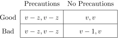
1.2.2 An Alternative Interpretation
There is an alternative interpretation of the model. Suppose that there are some costly precautionary measures that can be initiated by the agent if the principal forces him to do so. From the principal’s point of view, these precautions are necessary in case the project is bad since they completely eliminate the harms; otherwise, they are wasteful. The agent wants to avoid these measures regardless of the type of the project, due to the costs. Let z
Precautions No Precautions
Good v−z, v−z v, v
Bad v−z, v−z v−1, v
Table 1.1: Description of the corresponding payoffs at the ex-post stage for the principal and the agent respectively.
When z =v, the above description is equivalent to the baseline model, where forcing the precautions corresponds to the rejection of the project, and vice versa. However, the results of the paper also follow for a larger set of z values. One just needs to make sure thatz is not very different from v.10
1.2.3 Policy
The principal is endowed with the full commitment power, and, at t = 0, commits to a dynamic policy that specifies delegation and approval decisions over time as a function of the public history. The public history consists of information about the realized decisions in the earlier periods as well as the self-monitoring outcomes for those periods in which the monitoring is delegated to the agent.
For a given time period t, the corresponding delegation decision and the realized out-come of the self-monitoring, if performed, are denoted together by rt ∈ {s, ns, n}. When
monitoring is delegated to agent, rt will be either “s”, if self-disclosure takes place; or will
be “ns”, if no self-disclosure takes place. If there is no delegation, then rt=n. Moreover,
the approval decision at timet is denoted bydt∈ {0,1}, where 0 and 1 indicates rejection
and approval respectively. Consequently, a within-period public history, at the end of the period, which is denoted byht, is of the following form:
ht= (rt, dt)∈ {s, ns, n} × {0,1},
10For instance, whenzis sufficiently small, then the principal would always force these measures and avoid
for each t. At the beginning of a period t, a public history is defined as
ht= (h1, ..., ht−1).
The initial history is h1 =h0 =∅, and Ht is the set of public histories at period t.
A policy Γ ={γt, xt}∞t=1 is then a sequence of functions which are defined as follows:
γt:Ht→[0,1],
xt:Ht× {s, ns, n} →[0,1].
The functionγt is the probability of delegation. Because the delegation takes place at the
beginning of each period, it is a function defined over the set Ht. On the contrary, the approval decision is also conditioned on the value ofrt, hence the relevant domain forxt is
Ht× {s, ns, n}. For each possible value ofrt, I use a separate notation for the approval rate,
i.e., xt= (xst, xnst , xnt). Note that,xst andxnst are well-defined as long asγ >0; similarlyxnt
is relevant whenγ <1.
For an incentive compatible policy Γ, the expected utilities of the principal and the agent are denoted by V andU respectively, and are given by:
U =E
h
(1−δ)
∞
X
t=1
δt−1γt{µλxstv+ (1−µλ)xnst v−c}
| {z }
Delegation
+ (1−γt)xntv
| {z }
No Delegation
i
V =E
h
(1−δ)
∞
X
t=1
δt−1γt{µλxst(v−1) + (1−µλ)xnst (v−µns)−c}
| {z }
Delegation
+ (1−γt)xnt(v−µ)
| {z }
No Delegation
i
other case will be analyzed later on.
1.2.4 Stationary Representation
Following Spear and Srivastava (1987), I express the principal’s problem within a stationary form, in which the ex-ante expected utility of the agent is the state variable. In this form, the interval [0, v] is the corresponding state space as it consists of all of the possible values that the ex-ante expected utility of the agent can take. The agent’s utility cannot be negative, because he can always guarantee a non-negative utility by shirking every time he is asked to monitor. On the other hand,vis the maximum that the agent can receive in a policy. The principal can grant this maximal utility to agent by approving all of the projects without requesting self-monitoring.
State variable is updated over time depending on the realized public history. Within-period decisions and the promised future continuation utilities of the agent, depend on this state variable as well as the realized outcomes of the current period. An optimal policy specifies a different continuation utility for each possiblert∈ {s, ns, n} as in the case of the
approval probabilities. More precisely, the components of the policy are defined as:
γ, xs, xns, xn : [0, v]→[0,1],
Us, Uns, Un : [0, v]→[0, v].
The delegation and the approval decisions consist, in essence, of probabilities; therefore, the functions γ, xs, xns, xn take their values from the unit interval. The continuation
utili-ties, on the other hand, specify the state variable for the next period; hence, they are defined as functions from the state space to itself. For a given policy, the functionsUs, Uns, xs,and
xnsare relevant only for those values ofU ∈[0, v] satisfyingγ(U)>0, whereas the functions
The promised utility of the agent is calculated in ex-ante terms; hence, it will be granted to the agent only in expectation. It aggregates the flow and continuation utilities of the agent. Its transition is governed by the policy and the stochastic realizations. Starting fromU, the state variable of the next period becomesUn(U), orUs(U), orUns(U) with the
corresponding probabilities 1−γ(U),γ(U)µλ and γ(U)(1−µλ) respectively.
In an optimal policy, the functionsUn, Us, Uns, γ, xn, xs, xnsare chosen to maximize the
principal’s objective function. There are two constraints that the principal needs to take into account in this problem: incentive constraint and promise keeping constraint. More precisely:
1.2.5 Principal’s Problem P
V(U) = max
γ, xn,xs,xns, Un,Us,Uns
γhµλ
(1−δ)xs(v−1) +δV(Us)
+ (1−µλ)
(1−δ)xns(v−µns) +δV(Uns)
−ci
+(1−γ)h(1−δ)xn(v−µ) +δV(Un) i
subject to the (PK) and (IC) respectively:
U =γhµλ
(1−δ)xsv+δU s
+ (1−µλ)
(1−δ)xnsv+δUns
−ci+ (1−γ)h(1−δ)xnv+δUn i
,
γhµλ(1−δ)xsv+δU s
+ (1−µλ)(1−δ)xnsv+δUns
−ci≥γh(1−δ)xnsv+δUns i
.
The first line of the principal’s objective function includes her utility contingent upon self-monitoring request; hence, it is multiplied by the probabilityγ. The second line, on the other hand, corresponds to the contingency of no self-monitoring; hence, it is multiplied by 1−γ.
utility, the agent’s utility also has two components depending on the principal’s delegation decision.
The second constraint is the incentive constraint, which is defined to make sure that acquiring information is an optimal choice for the agent when he is asked to do so; hence, it is relevant only if γ >0. It guarantees that the utility the agent achieves from shirking is no better than the promised utility. If he shirks, there is no self-disclosure; hence, the current approval rate and the continuation utility will be equal toxnsand Unsrespectively.
Note that Blackwell’s sufficiency conditions, i.e., monotonicity and discounting, are fulfilled. Therefore, the existence of a solution for the problem P is guaranteed.
1.3
Case 1: Principal Internalizes Cost
In this section, I study the optimal policy and its properties under the first preference specification, i.e., when the principal internalizes the self-monitoring costs. First, I start with a benchmark analysis.
1.3.1 Observable Information Acquisition
w andπ respectively, and are given by:
w= (1−µλ)v−c,
π= (1−µλ)(v−µns)−c.
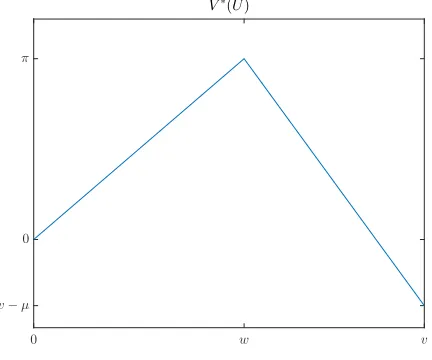
The optimal policy when the self-monitoring effort is observable induces the first best out-come, which gives the maximum possible utility to the principal. What about the optimal policy conditional on the agent receiving a certain utility U ∈[0, v] when the effort is ob-servable? To answer this question, one needs to solve the same problemP without including the incentive constraint. This problem has a solution, and the value function arising from its solution, which I denote by V∗, is an upper-bound for the value functionV.
To describeV∗ and the corresponding “benchmark policy”, I will point out some initial observations. First of all, the benchmark policy is stationary without loss of generality. The expected utility of the agent stays constant throughout time; and hence, one just needs to characterize the delegation and the approval decisions, which I denote byγ∗, x∗n, x∗s, x∗ns, as functions ofU ∈[0, v].
Second, the information must be used efficiently. In other words, whenever the agent is asked to monitor himself, the following approval decision must be efficient conditional on the content of the resulting information. This is a direct implication of the fact that the principal internalizes the self-monitoring costs. Rather than having x∗s >0 or x∗ns<1, the principal could adjust the probability of delegation, γ∗, without hurting the promise keeping constraint, and get strictly better off. To see this, first note that:
U =γ∗[µλx∗sv+ (1−µλ)x∗nsv−c] + (1−γ∗)x∗nv.
Suppose, xs > 0 to get a contradiction, then it must be true that xns = 1; because,
otherwise, there is an immediate deviation that the principal can perform by decreasing x∗s
probability to γ −ζ. Moreover assume that the principal employs a direct approval with the remaining ζ probability. Then ζ satisfies:
γ∗[µλx∗sv+ (1−µλ)v−c] = (γ∗−ζ)[µλ(x∗s−)v+ (1−µλ)v−c] +ζv.
Therefore:
ζ = γµλv
µλv(1−xn+) +c
.
Such a deviation is strictly better for the principal, because:
h
(γ∗−ζ)[µλ(x∗s−)(v−1)+(1−µλ)(v−µns)−c]+ζ(v−µ) i
−hγ∗[µλx∗s(v−1)+(1−µλ)(v−µns)−c] i
>0.
A similar contradiction follows for the case x∗ns<1.
Finally, upon not requesting self-monitoring, the principal either directly approves or directly rejects the projects and not chooses a randomized approval decision. Instead of choosing an x∗n∈(0,1), she could increase the probability of delegation, γ∗, and adjust the value ofx∗n by respecting the promise keeping constraint. This increases the probability of informed decision making and improves the principal’s objective.
γ∗(U) =
U
w ifU ∈[0, w] v−U
v−w ifU ∈(w, v]
x∗s = 0, x∗ns= 1, ∀U ∈(0, v)
x∗n(U) =
0 ifU ∈[0, w) 1 ifU ∈(w, v] And the resulting value function is:
V∗(U) =
U
wπ ifU ∈[0, w]
v−U v−wπ+
U−w
v−w(v−µ) ifU ∈(w, v]
The following figure illustrates the value function.
0 w v
v−µ
0
π
V∗(U)
1.3.2 Moral Hazard and The Optimal Policy
The focus is now on the agency problem where the agent’s efforts spent on self-monitoring are not observed by the principal. The interest is particularly on the characterization of the value functionV, within-period decisions γ, xn, xs, xns, and the promised continuation
utilitiesUn, Us, Uns, which are defined as functions of the ex-ante expected promised utility
U. The following lemma, which is proved in appendix, is a first step towards this goal.
Lemma 1.1. The value function, V is concave and hence differentiable almost everywhere.
Moreover its derivative is bounded and satisfies:
1− µλ
µλv+c ≤V
0(U)≤1− µ(1−λ)
(1−µλ)v−c, ∀U ∈[0, v]. (1.1)
Proof. See appendix A.1.
The concavity of the value function is a direct implication of the fact that the principal can randomize between different utility levels while granting a specific promised utility to agent. Since V is concave, it is almost everywhere differentiable, which can also be proved by applying the result of Benveniste and Scheinkman (1979). The following observations are sufficient to show the bounds of the derivative ofV. First, for any promised utility U,
V(U) cannot be larger thanV∗(U). Second, the values ofV andV∗ are equal to each other at the boundaries of the state space, i.e., at 0 and v. These observations together with the concavity require that the constant slopes ofV∗ over the intervals [0, w] and [w, v] are the upper and the lower bounds ofV0 respectively.
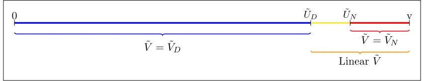
her promises in expectation. Otherwise, the principal, in each period that she is supposed to randomize, could pick the outcome that she prefers most instead of following the specified randomization.
In this regard, one can represent the utility of the agent as a weighted average of two components, one for each possible outcome of the delegation decision. Precisely, letUD and
UN be the resulting utilities of the agent after delegation and no delegation respectively.
More precisely:
UN = (1−δ)xnv+δUn
UD =µλ
(1−δ)xsv+δU s
+ (1−µλ)
(1−δ)xnsv+δUns
−c.
The promise keeping constraint imposes a restriction on the choices of UD,UN, andγ, so
that the equality U = γUD + (1−γ)UN must hold. When the agent is delegated with
certainty, i.e whenγ = 1, it must be U =UD; similarly, U =UN must hold when γ = 0.
1.3.3 Conditional Representation
In what follows, I will further exploit the above-mentioned observation, and rewrite the principal’s problem P as a decomposition of two conditional programs. These sub-programs are defined conditional on the current delegation decision, and their task is to characterize the approval decision in the current period as well as the continuation utilities for the next period.
The first problem is defined conditional on principal delegating monitoring to the agent in the current period. The solution to this problem characterizes the optimal values forxns,
xs,Uns, andUsdepending on the value ofUD. It incorporates the incentive constraint and
The second program is defined conditional on agent not delegating monitoring to the agent in the current period. Its solution characterizes the optimal values of xn and Un
depending on the value of UN. There is no incentive constraint in this problem, since there
is no request of self-monitoring. There is only a promise keeping constraint defined to make sure thatxn and Un are arranged so that the agent’s utility is equal toUN.
Conditional on no delegation, the agent’s utility can take all the values in the entire state space, hence the range of UN is equal to [0, v]. However, this is not the case for UD.
It is defined conditional on an incentive compatible self-monitoring in the current period; hence, the agent already assumes the cost c. This means that UD cannot be equal to v or
anything sufficiently close to v; therefore, the range of UD can only be a proper subset of
the state space. The exact range ofUD will be discussed later on.
The corresponding value functions arising from these conditional programs are denoted by VD and VN respectively. The unconditional value function, V, is then given by:
V(U) =γ(U)VD(UD) + (1−γ(U))VN(UN),
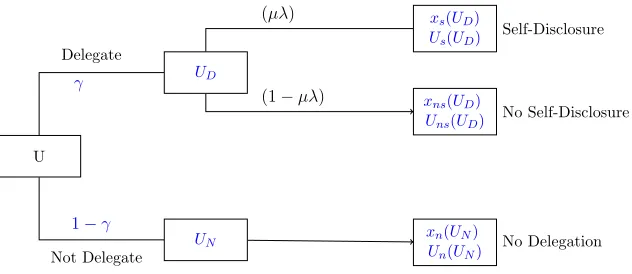
where U = γ(U)UD + (1−γ(U))UN. The following diagram illustrates this conditional
representation of the principal’s problem.
U
UD
UN
xs(UD)
Us(UD)
xns(UD)
Uns(UD)
xn(UN)
Un(UN)
Self-Disclosure
No Self-Disclosure
No Delegation γ
Delegate
1−γ
Not Delegate
(µλ)
(1−µλ)
Figure 1.3: The principal’s problem is equivalent to solving for the optimal values of UD,
This new form of the principal’s problem is denoted byP0 and it is defined as follows:
V(U) = max
γ,UD,UN γVD(UD) + (1−γ)VN(UN),
s.t. U =γUD+ (1−γ)UN.
The sub-program that is conditional on no delegation in the current period is denoted by
PN, and is defined as follows:
VN(UN) = max
xn,Un[(1−δ)xn(v−µ) +δV(Un)],
s.t. UN = (1−δ)xnv+δUn.
Finally, the sub-program that is conditional on delegation in the current period is denoted asPD, and is defined as:
VD(UD) =xn,xs,xns,max Un,Us,Uns h
µλ(1−δ)xs(v−1) +δV(Us)
+ (1−µλ)(1−δ)xns(v−µns) +δV(Uns)
−ci
subject to (PKD) and (ICD) respectively:
UD =µλ
(1−δ)xsv+δU s
+ (1−µλ)(1−δ)xnsv+δUns
−c,
UD ≥(1−δ)xnsv+δUns.
Thanks to this conditional formulation, it is possible to analyze the principal’s delega-tion and approval decisions separately. First, I will consider the condidelega-tional problems in isolation, and solve for the corresponding optimal approval decisions. Then, I will focus on the unconditional problemP0, and characterize the optimal delegation decision over the
state space.
takes place between VD(UD) andVN(UN), thenV(UD) =VD(UD) and V(UN) =VN(UN).
In other words, γ = 1 is optimal at UD, and γ = 0 is optimal atUN. This observation is
based on the fact that the principal, in order to grant the agent his promised utilityU, can always randomize betweenV(UD) andVN(UN). Therefore,V(UD) cannot be strictly larger
thanVD(UD), as it would contradict with the optimality.
On account of this, characterizing the state variables that are featuring γ = 0 or
γ = 1 would be sufficient to pin down the optimal delegation decision. In other words, the focus should be on the subsets of the state space over which either V(U) =VD(U) or
V(U) = VN(U) is satisfied. For the rest of the state space, there will be a randomized
delegation decision, and the corresponding valuesUD and UN will always be a part of the
subsets of [0, v] satisfying V =VD and V =VN respectively.
The discussion in the sequel will follow the plan descrived above. In order to carry through the first step, I will first focus on the conditional problems in isolation.
1.3.4 The problem PD
An initial observation is that the incentive constraint is always binding. First of all, note that the IC can be written as a restriction on the difference between the continuation utilities
Us and Uns:
Us−Uns≥
1−δ δµλ c+
1−δ
δ (xns−xs)v.
In case the difference betweenUs andUns is larger than the value that is necessary to
maintain incentive compatibility, the principal can move them closer to each other without violating the promise keeping constraint. More precisely, she can decrease Us by and
increase Uns by 1−µλµλ. Such a modification is always feasible as long as > 0 is chosen
the principal due to the concavity of the value function V. This is because the suggested modification consists of a mean preserving contraction of the continuation utilities, hence the expectation of V for the next period becomes larger. Therefore incentive constraint is always binding, without loss of generality. Solving binding incentive constraint together with the promise keeping constraint gives:
Us=
UD
δ +
1−δ δµλ c−
1−δ
δ xsv, (1.2) Uns=
UD
δ −
1−δ
δ xnsv. (1.3)
These expressions suggest that the agent is compensated for the cost of information acquisition only after the signal is realized. To see this more clearly, one can rewrite them as follows:
(1−δ)xnsv+δUns=UD,
(1−δ)xsv+δUs=UD+1µλ−δc.
Self-reporting increases the agent’s utility by a constant. Since the signal is verifiable, it also serves as a proof of the effort spent on self-monitoring. Therefore, the most efficient incentive provision scheme involves compensating the agent for the costs of monitoring only after the realization of the signal. Another important aspect is that the continuation utility in one contingency is independent of the approval rate in the other contingency. In other words,Us is independent of the choice ofxns, and Unsis independent of xs.
After figuring out the relation between approval probabilities and the continuation utilities, it is now possible to discuss the domain of value function VD. By using the
equations (1.2), and (1.3), one can see that the maximum value thatUD can take is equal
toδv+(1−µλδ)c, which can be achieved by settingxs andUsequal to their maximum values,
To characterize the solution of the problemPD, one needs to use the equations (1.2), and (1.3) that govern the trade-off between the continuation utilities and the current approval rates for both contingencies, i.e., self-disclosure and no self-disclosure. The question is, to what extent the principal would like to use efficient approval decisions, i.e. xns = 1 and
xs = 0? It turns out that the approval decisions will be set as close as possible to the
efficient ones. More precisely, xs = 0 and xns = 1 as long as the resulting continuation
utilities, i.e., Us and Uns, stays inside the state space [0, v]. This requires UD to be in an
intermediate range. WhenUD is sufficiently small, settingxns= 1 is not feasible, since the
resultingUnswould be negative. For these values, the approval ratexnswill be chosen such
that the continuation utilityUnsbecomes 0. By the same logic, for those values ofUD that
are sufficiently large, the approval rate xs will be chosen so that the continuation utility
Us takes its largest possible value v. The formal statement of the lemma is given by the
following lemma.
Lemma 1.2. There exists critical values
¯
U = (1−δ)v, and U¯ =δv− (1−µλδ)c, such that the solution to the problem PD satisfies:
(xs, xns) =
(0,(1UD−δ)v) if UD ≤
¯
U,
(0,1) if UD ∈(
¯
U,U¯),
(UD+
(1−δ)c µλ −δv
(1−δ)v ,1) if UD ≥U.¯
(Us, Uns) =
(UDδ +(1δµλ−δ)c,0) if UD ≤
¯
U,
(UDδ +(1δµλ−δ)c,UD−(1δ−δ)v) if UD ∈(
¯
U,U¯),
(v,UD−(1δ−δ)v) if UD ≥U.¯
Proof. See appendix A.2.
decrease xs as much as possible due to the efficiency concerns. However, these approval
rates also alters the continuation utilities, therefore there is a non-trivial tradeoff that the principal needs to take into account. As can be seen from the equations (1.2), and (1.3), a higherxns requires a lower Uns, and a smallerxs requires a higherUns.
Lemma 1.2 proves that, even if there is a loss resulting from a lowerUns, the tradeoff
always favors a higher approval rate xns. Similarly, even if there is a loss resulting from
higherUs, the tradeoff always favors lowerxs. The lower and upper bounds of the derivative
of the value function V, which are defined in lemma 1.1, are the main driving force behind this result. Precisely, the upper and lower bounds ofV0 puts a limit on the maximum loss that can arise, and this limit is always less than the gain from employing more efficient approval decisions. Note that theU < U¯ is always satisfied due to the restriction imposed on the discount factor δ.
1.3.5 The problem PN
This problem is defined conditional on no delegation in the current period. Its solution follows from straightforward arguments. The decision is mainly about how much of the promised utility, UN, to provide the agent in the current period in the form of project
approval, and how much of it to leave as a continuation utility. The amount that is left as a continuation utility will be granted to the agent starting from the next period without any restriction on the delegation decision. The optimal choice of the approval rate follows from the following maximization problem.
max
xn (1−δ)xn(v−µ) +δV(
UN−(1−δ)xnv
δ ).
on Un. LetI = [
¯
a,¯a] be an interval where the boundaries
¯aand ¯asatisfy:
¯
a= inf{U ∈[0, v]|V0(U)≤ v−µ
v },
¯
a= sup{U ∈[0, v]|V0(U)≥ v−µ
v }.
In words, I is the interval over which the derivative of the value function V is equal to v−vµ. This interval resides in the interior of the state space [0, v]. This stems from the fact that, the line that connects the points (0, V(0)) and (v, V(v)) has the slope v−vµ, and the graph of the value function V locates over this line.11 Then due to the concavity,
V0(0)> v−vµ > V0(v), hence the intervalI is in the interior of the state space [0, v].12 Then, one can conclude that the optimal choice ofxnsatisfies the following:
xn(UN) =
0 ifUN ≤δ
¯
a,
∈(0,1) ifUN ∈(δ
¯a, δ¯a+ (1−δ)v), 1 ifUN ≥δa¯+ (1−δ)v.
(1.4)
Intuitively, for smaller values ofUN, the continuation valueUnwill be in a range where
the derivative of V is sufficiently large. In this region, it is better for principal to keep the continuation utility as high as possible by setting xn = 0. On the contrary, for larger
values of UN, the value of V0 becomes small, and increasing the continuation utility does
not benefit the principal. Therefore, she keeps the continuation utility of the agent as small as possible by settingxn= 1.
In the intermediate range ofUN, however, the value ofxnis set so that the continuation
value lies in the intervalI, and hence the value function has a derivative equal to v−vµ. The principal is indifferent between marginally increasing xn and Un. If the interval I consists
11
The linear line can be achieved by an always feasible policy: randomizing between its extreme values. Hence it is strictly dominated, andV stays on top of this line.
12
of a single point, then the optimal value of xn is also singleton. Otherwise, there is a
continuum of optimal values forxn in this intermediate range.
1.3.6 The problem P0
From now on, the conditional problems PD and PN will be considered together in order to characterize the solution of the unconditional problem. The task is to figure out the optimal way to decompose U into UD and UN together with the the optimal choice of γ.
Completing these tasks will lead to the description of the value functionV, which is equal to the concavification of the functionsVD and VN.13
The following lemma describes the set of state variables over which the equalityV =VN
is satisfied. It further indicates that the corresponding approval rates at these state variables must be either 0 or 1. In other words, having an interior probability of approval, i.e.
xn∈(0,1), after avoiding self-monitoring never happens in an optimal policy.
Lemma 1.3. There are two critical values 0<
¯
UN <U¯N < v, such that:
i) V(U) =VN(U) if and only if U ∈[0,
¯
UN]∪[ ¯UN, v]
ii) V is linear over [0,
¯
UN] and[ ¯UN, v].
iii) The optimal approval decisionxn satisfies:
xn(U) =
0 if U ∈[0,
¯
UN]
1 if U ∈[ ¯UN, v]
Proof. See appendix A.3
13The value functionV depends onVD andVN, which in turn depend onV. In this regard,V,VD, and
Lemma 1.3 points out that making an uninformed decision without monitoring can be optimal only if the promised utility is close to the boundaries of the state space. It is already known that the equality V = VN holds at the extreme values of the state space,
i.e., at 0 and v. By using the comparison between the VN0 and V0, which can be achieved from the equation (1.4), one can show that the equality V = VN can hold only over the
union [0, δ
¯
a]∪[δa¯+ (1−δ)v, v]. Then by using the expression (1.4), one can conclude that the approval probability xn must be either 0 or 1 for all the promised utilities at which
no-delegation is optimal. The second step of the proof shows the existence of the cutoffs ¯
UN, and ¯UN, and also the fact that they reside in the interior of the state space.
This result is rather intuitive. When U is sufficiently low, it is not feasible to utilize a large approval rate; similarly, whenU is sufficiently large, it is not feasible to employ a large rejection rate. Therefore, the principal can get only limited benefit from the information in these state variables, and the extent of this benefit is not sufficient to compensate the cost of acquisition. For this reason, she does not ask the agent to self-monitor at these promised utilities as she also cares about the costs. Therefore, no-delegation is an optimal solution, and henceV =VN holds.
The result is also informant about the shape of the value function over the lower and upper ends of the state space, as it points out that the value functionV is linear over the intervals [0,
¯
UN], and [ ¯UN, v]. Following some simple logic, one can see that the linearity is
not limited to these intervals. More precisely:
V(U) =VN(U) =
δV(Uδ) ifU ∈[0,
¯
UN]
(1−δ)(v−µ) +δV(U−(1δ−δ)v) ifU ∈[ ¯UN, v]
V0(U) =VN0(U) =
V0(Uδ) ifU ∈[0,
¯
UN]
V0(U−(1δ−δ)v) ifU ∈[ ¯UN, v]
SinceV0(U) =V0(Uδ) for everyU ∈[0,
¯
UN], andV is concave, the slope is constant over
[0,
¯
UN]∪[
¯
UN,UN¯δ ]. Similarly, the slope ofV is constant over [ ¯
UN−(1−δ)v
δ ,U¯N]∪[ ¯UN, v]. Due
to the linearity of the value function, it is without loss of generality to assume that there is a randomized delegation decision over the intervals (
¯
UN,
¯
UD) and ( ¯UD,U¯N).
The constant slopes, however, does not carry beyond the values ¯UNδ , and UN¯ −(1δ−δ)v.14
As a result, no randomized delegation decision can be optimal at these values, since they do not have any neighborhood over which the slope of V stays constant. At these values,
γ = 0 can not be optimal either, because it is already known that VN < V for all of the
state variables that are outside of [0,
¯
UN]∪[ ¯UN, v] form the previous lemma. As the only
remaining option, the equalityV =VD must hold at these values. To this respect, one shall
define:
¯
UD = ¯
UN
δ
¯
UD =
¯
UN −(1−δ)v
δ
The values ¯
UD, and ¯UD are the smallest and largest values of U satisfying V(U) =VD(U)
without loss of any generality. The interval ( ¯
UD,U¯D) is the only remaining region where
the delegation decision is yet to be described. However, it is natural to expect thatV =VD
and henceγ = 1 over ( ¯
UD,U¯D).
Let U ∈ ( ¯
UD,U¯D). From lemma 1.3, VN < V, and hence γ >0 at this U. Moreover,
a randomized delegation decision cannot be optimal either. Suppose otherwise to get a contradiction, and assume that a randomization takes place betweenVD(UD) andVN(UN).
14
IfV0 were to be constant on any neighborhood of ¯U
δ and
¯
UN−(1−δ)v
δ , then the equalityV =VN would hold for a larger subset of [0, v], which contradicts with the definition of
¯
The corresponding value ofUN must belong to either [0,
¯
UN] or [ ¯UN, v]; without loss of
gen-erality assume the precedent. Then, the principal could rather randomize between VD(
¯
UD)
and VD(UD) and get strictly better off. The reason for this stems from the fact that slope
ofV alters at ¯
UD, hence the line connecting the valuesVD(UD) andVD(
¯
UD) locates on top
of the line connectingVD(UD) andVN(UN). Therefore, it is optimal to setγ= 1 and hence
V =VD in this region.
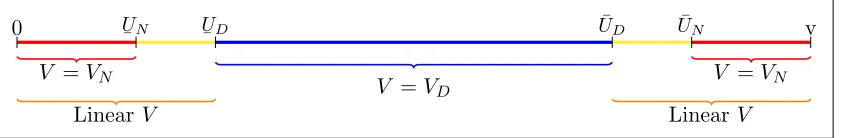
The optimal delegation decision for each possible promised utility U ∈ [0, v] is now known, and summarized in the following diagram:
0 ¯UN
¯
UD U¯D U¯N v
V =VN V =VN
V =VD
Linear V LinearV
Figure 1.4: Partition of the state space depending on the optimal delegation decision.
To complete the characterization of the optimal policy, one should also describe the approval decisions. Particularly, the description of xs and xns over the interval [
¯
UD,U¯D],
where delegation is the optimal choice, is incomplete.
The problem PD is analyzed in isolation, and its solution is provided in lemma 1.2.
The result asserts that the efficient decision making, i.e. xs = 0, and xns = 1 will take
place as long as the promised utility U is in between [ ¯
U,U¯]. For the rest of the state space, making the efficient decisions is not feasible. Instead, the principal employs the decisions that are closest to the efficient among the feasible ones. However, the problemPD is defined conditional on delegation in the current period regardless of its optimality. Now, the focus is on the interval [
¯
UD,U¯D], where delegating monitoring is optimal.
The question one shall inquire at this point is, how do the values of ¯
UD, and ¯UD
compare to the values of ¯