Bettinger

(1)

ONE YEAR’S EXPERIENCE WITH A RECREATION-GRADE GPS

RECEIVER

Pete Bettinger

1

, SongLin Fei

2

,

1_{Professor, WSFNR, University of Georgia, Athens, GA 30602 USA} 2 _{Asssistant Professor, University of Kentucky, Lexington, KY 40506 USA}

Abstract.Between September 2008 and September 2009, data were collected with a Garmin Oregon 300

recreation-grade GPS receiver nearly every day, under a variety of environmental conditions. Horizontal position locations were collected in a young pine stand, an older pine stand, and a hardwood stand, each located within the Whitehall Forest GPS Test Site in Athens, GA. The purpose of this study was to determine whether long-term data collected with a recreation-grade GPS receiver were sensitive to stand type, time of year, and a number of environmental variables. We found no significant relationship between observed horizontal positional accuracy and environmental variables (air temperature, relative humidity, atmospheric pressure, and solar wind speed). We found significant differences in horizontal position accuracy among the three forest types studied.

Keywords:Global positioning systems, root mean squared error, horizontal position accuracy

1 Introduction

Satellite positioning systems are a pervasive technol-ogy in forest management. The desire for highly accu-rate locational information is understandable, and this technology is slowly replacing traditional navigation and mapping techniques. A number of research projects have evaluated the ﬁtness of GPS technology for forestry use (e.g., Gerlach and Jasumback 1989; Evans et al. 1992; Veal et al. 2001, Wing et al. 2005, 2008, Danskin et al. 2009a, 2009b). These and other studies continue to provide forest managers assessments of GPS positional accuracy under forested conditions. However, given the rapid changes in technology, a continuous review seems necessary. In addition, the potential issues of environ-mental variables on GPS positional accuracy need to be more fully understood to encourage forest managers to integrate it into their daily operations.

The United States Global Positioning System (GPS) currently consists of 31 satellites, with a minimum of four in each of six orbital planes around the Earth. Each satellite broadcasts a unique signal that can be acquired by commercially-available GPS receivers on the L1 fre-quency (1575.42 MHz) through the coarse acquisition (C/A) code. By utilizing the time of arrival associated with of these signals, the distance from a GPS receiver to each satellite can be determined, and a position can be trilaterated. While most current GPS receivers can track

eight or more satellites at one time, with four satellite signals, both horizontal and vertical positions can be es-timated. The performance of GPS receivers in forested environments is aﬀected, however, by topography and vegetation (Danskin et al. 2009b). Vegetative obstruc-tions can play a signiﬁcant role in introducing error into position estimates through the blocking of satellite sig-nals (thus forcing the use of less valuable sigsig-nals) or through the use of multipathed signals (those being redi-rected from the ground or other nearby features).

Throughout the literature and in practice, GPS receivers are divided into three general classes: survey-grade, mapping-grade, and recreation-grade (or consumer-grade). Survey-grade GPS receivers are capa-ble of providing sub-centimeter horizontal position accu-racy in open areas, and sub-meter accuaccu-racy under forests (Danskin et al. 2009a). However, at a cost of $10,000 dollars or more, these GPS receivers are not typically available for general forest management use, and if avail-able, may be too bulky or heavy to carry around in the woods. Mapping-grade receivers are capable of provid-ing sub-meter accuracy in open areas and 2-5 m accu-racy in forested conditions. These range in price from about $1,000 to $5,000, and are frequently used in for-est management. Recreation-grade receivers provide the least accurate horizontal position accuracy, generally in the 5-15 m range, and vary in price from $100 to $600.

(2)

Recreation-grade receivers are popular among foresters and other outdoors enthusiasts, yet while not typically used for land mapping purposes, they are used for mark-ing the position of research plots and wildlife censusmark-ing stations (among others). The choice of GPS receiver to use depends on the anticipated application(s), and an organization’s cost considerations. When single-fix posi-tional errors of 5-15 m are acceptable, a recreation-grade GPS receiver would suffice. A recreation-grade GPS re-ceiver may be acceptable for locating field points when one knows they will be in one location for some time (allowing the capture of multiple fixes). Ultimately, the cost of data collection and the desired accuracy levels of referenced positions should be balanced.

The objectives of this work were to understand how GPS positional accuracy levels change over the course of a year given variation in environmental conditions. One set of hypotheses suggests that GPS positional accuracy would not change as environmental conditions (air tem-perature, relative humidity, etc.) change, with the GPS receiver studied. Another set of hypotheses suggests, based on prior research results, that GPS positional ac-curacy would be significantly different for the different forest types under consideration. Further, another set of hypotheses suggests, based on prior research results, that there would be differences in GPS positional ac-curacy across seasons of the year within a single forest type.

2 Methods

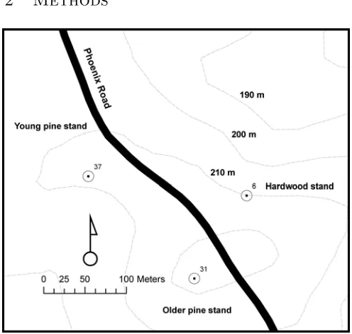
Figure 1: A map of the three Whitehall Forest GPS Test Site points used in this research.

Three test points (numbers 6, 31, and 37) from those

available at the Whitehall Forest GPS Test Site in Athens, GA (http://warnell.forestry.uga.edu/Warnell/ Bettinger/GPS/UGA GPS.htm) were selected for this research (Figure 1). Test point 37 is located in a young loblolly pine (Pinus taeda) plantation (15 years old, 130 ft2_{per acre basal area, 450 trees per acre, southwest}

as-pect, 8% slope, 212 m elevation, 95% canopy closure). Test point 31 is located in an older loblolly pine stand (60-70 years old, 86 ft2 _{per acre basal area, 59 trees}

per acre, south aspect, 2% slope, 222 m elevation, 50% canopy closure). Finally, test point 6 is located in an older hardwood stand (60-70 years old, 88 ft2 _{per acre}

basal area, 144 trees per acre, northeast aspect, 18% slope, 210 m elevation, 90% canopy closure in the sum-mer, 40-50% canopy closure in the winter). The older hardwood stand around test point 6 is dominated by oak (Quercusspp.) and hickory (Caryaspp.). All three test points are located in upper slope positions, and repre-sent the best choices for comparison among the three forest types. The three test points were visited once per test day (289) over the course of a year (Septem-ber 15, 2008 to Septem(Septem-ber 14, 2009), and ﬁfty position ﬁxes were collected at each test point during each visit. The order of visit to each of the three test points was randomized each day. Travel time between test points required about 3 minutes.

The number of position fixes to collect at each visit has been extensively explored by others. Our assump-tion (50 posiassump-tion fixes) is consistent with recent studies (Danskin et al. 2009a, 2009b, Wing 2008, Wing et al. 2008). Sigrist et al. (1999) suggested that 300 posi-tions fixes per control point were necessary, and Deck-ert and Bolstad (1996) concluded that error decreases when more position fixes are acquired. However, Wing (2008), who sampled up to 60 position fixes per visit to a control point, found that the number of fixes was signif-icant in only one-third of the consumer-grade receivers tested. Wing et al. (2008) further suggest that 30 fixes per point position seemed to be appropriate for highly accurate measurements when using mapping-grade GPS receivers. Although a consumer-grade receiver is used in this study, we found that 50 position fixes were appro-priate, as we outline in the results.

(3)

available 100% of the time, and the GPS receiver was unable to record whether the system was being used at any one point in time. The recording of position fixes (waypoints) was performed manually, with 2-3 second elapsing between fixes. We were unable to use a stan-dard period of time between position fixes, because the GPS receiver did not have the ability to automate data collection. At the beginning of each day’s visit, some warm-up time (up to five minutes on occasion) was re-quired to ensure that a sufficient number of satellites were available to provide a reasonable position fix. Dur-ing each visit, the GPS receiver was plumbed directly over each test point (using a staff and a plumb bob), and the lead investigator stood on the north side of each as data was collected.

Planned PDOP (Positional Dilution of Precision) for the period of data collection was acquired using Trim-ble GPS planning software; actual PDOP data was un-available from the GPS receiver studied. PDOP is a measure of the eﬀect of GPS satellite geometry on GPS precision, and a low value is generally representative of better GPS positional precision because of the wider angular separation between the GPS satellites that are used to determine a position on the ground. Weather data (air temperature, relative humidity, atmospheric pressure) for the Athens, GA area at the time of each visit were derived from Internet sites. In lieu of in-stalling our own weather station at the GPS test site, we derived weather data from the Internet sites of the Weather Channel and Weather Underground. These sites usually report weather in 15-20 minute intervals, and given the 15-20 minute per day sampling regimen, we determined the mid-point sampling time and de-veloped a weighted average of the weather values sur-rounding this time frame. Solar wind speed (HE++ velocity, in km/second) was also considered, since so-lar outbursts might interfere with GPS signals. So-lar wind speed data was derived from CalTech’s Ad-vanced Composition Explorer (ACE) Science Center (http://www.srl.caltech.edu/ACE/ASC/). GPS data were downloaded from the Garmin Oregon 300 using Minnesota DNR Garmin software (Minnesota Depart-ment of Natural Resources 2001). Data were then trans-ferred to a database for further analysis.

We subdivided the data by the season in which it was collected. For our purposes, the fall season covered the period from September 15, 2008 to December 14, 2008. The winter season covered the period from December 15, 2008 to March 14, 2009. The spring season covered the period from March 15, 2009 to June 14, 2009. The summer season covered the period from June 15, 2009 to September 14, 2009. GPS data were collected between 10:30 AM and 4:30 PM, depending on the schedule of the lead researcher. A consistent time throughout the year

was nearly impossible to schedule, given other responsi-bilities. For example, the average Coordinated Universal Time (UTC) for the onset of data collection in the older pine stand was 19:45 in the fall season, 19:40 in the win-ter season, 18:11 in the spring season, and 17:04 in the summer season. Variation in sampling times increased with spring and summer seasons due to changes in the lead researcher’s teaching schedule. The standard de-viation, for example, for the onset of data collection in the older pine stand was 47.0 minutes in the fall season, 91.1 minutes in the winter season, 123.9 minutes in the spring season, and 116.8 minutes in the summer season. The eﬀect of these trends is unknown at this time on the results, however major diﬀerences in data collection times (e.g., almost always in the afternoon in the fall season, or almost always in the morning in the spring season) were not present.

The accuracy of horizontal positions was calculated using the root mean squared error (RMSE), which can be calculated with:

RMSE = n i

((x_i−x_T)2_{+ (}y

i−yT)2₎/n ₍₁₎

wherenis the total number of observations in a visit,i is the ith observation of the visit (i = 1 ton), x_i and

yi is the longitude and latitude of the ith observation, respectively, and x_T and y_T is true longitude and lati-tude of the test point. RMSE places a greater weight on the larger errors since the error term is squared. From the 50 position fixes collected each day under each forest type, one RMSE value was calculated for each day. These daily RMSE values were used along with the weather conditions in the statistical analysis. From a number of different perspectives (whole year, by season, within stand type, etc.), the RMSE values were not nor-mally distributed; therefore a log transformation was ap-plied prior to performing statistical tests of significance. Durbin-Watson test was then applied on log-transformed RMSE to examine if it is temporally autocorrelated. The Durbin-Watson test indicated no evidence of au-tocorrelation among the daily log-transformed RMSE. To understand the effects of forest type, season, and weather on GPS accuracy, an ANCOVA model analysis was conducted in SAS 9.2 (SAS Inc. Cary, NC). Log-transformed daily RMSE was set as the response vari-able, forest type and season were set as fixed factors, and weather variables (i.e., air temperature, relative hu-midity, atmospheric pressure, and solar wind speed) and planned PDOP were set as covariates. A variable was considered to have significant effect on RMSE if the modeledp-value is less than 0.05.

(4)

Table 1: Range of data accuracy over an entire year measured by root mean square error (RMSE) using a Garmin Oregon 300 GPS receiver.

Forest type Best RMSE (m) Worst RMSE (m) Mean RMSEa (m) Median RMSE (m)

Young pine (15 years old) 0.5 38.2 11.9 (A) 11.5

Older pine (60-70 years old) 0.2 46.2 6.6 (C) 5.8

Hardwood (60-70 years old) 0.8 28.7 7.9 (B) 7.3

a _{Mean RMSE values not sharing the same letter (A, B, or C) are signiﬁcantly diﬀerent at}_{p <}_0.05.

mean (RSEM). RSEM can be calculated with:

RSEM =

(

n

i

xi/n−xT)2+ ( n

i

yi/n−yT)2 (2)

RSEM is more closely comparable to results that one may obtain when using a mapping-grade GPS receiver for point data collection. Diﬀerences between RMSE and RSEM were examined by season and by forest type.

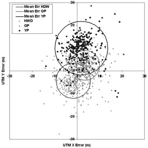
Figure 2: RMSE values for each visit to each forest type, and direction of error.

3 Results

Among all the variables measured, forest type is only variable that has a significant effect on RMSE (p < 0.01). Annual mean RMSE values were significantly dif-ferent among forest types (Table 1). The annual mean RMSE value was best (6.6 m) in the older pine stand, yet

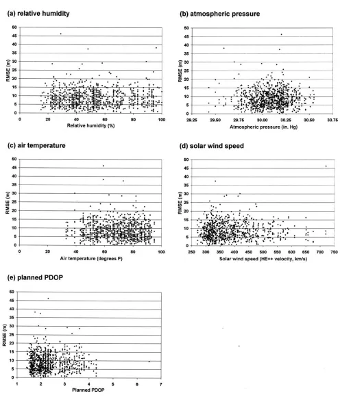
ranged from 0.2 m to 46.2 m on any one visit. The aver-age RMSE value for the hardwood stand (7.9 m) was a close second, and ranged from 0.8 to 28.7 m. The range of data accuracy in the young pine stand, for the entire year, was between 0.5 m and 38.2 m, and averaged 11.9 m. There also seemed to exist some interaction with the position of individual trees in each stand with regard to the location of the test points (Figure 2), since we are conﬁdent that the test point horizontal positions are known to within about 1.5 cm. Further research on these individual tree interactions could be tested using tempo-rary test points scattered in various fashions about the established test point, yet we leave this for others to in-vestigate in the future. No statistically signiﬁcant asso-ciations were found between horizontal positional error (RMSE) and relative humidity (Figure 3a), atmospheric pressure (Figure 3b), air temperature (Figure 3c), so-lar wind speed (Figure 3d), and planned PDOP levels (Figure 3e).

Contrary to other studies conducted on the same site, yet using different GPS technology, we found no differ-ence within a single stand type across seasons of the year with the Garmin Oregon 300 GPS receiver (Ta-ble 2). However, some findings are consistent with one of our hypotheses. For example, the mean and median RMSE values for the hardwood stand was lower in the winter than in the other seasons. This suggests that the satellite signals are stronger once they reach the re-ceiver, and thus the noise is lower, when the leaves are off of the hardwood trees. However, the mean and me-dian of the RMSE values in the older pine stand were lower in the spring and summer seasons than in the fall and winter. Further, the mean and median RMSE val-ues for the young pine stand were higher in the winter season than in the other seasons. Given that some pine needles would have been shed by the time of the win-ter season, it seems that the branches, rather than the needles, may have played a larger role in obscuring GPS signals in the pine stands. Again, while these results are interesting and are contrary to our proposed hypotheses, the differences among seasons within a single forest type were not significantly different.

(5)

(6)

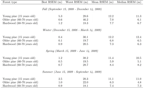
Table 2: Data accuracy measured by root mean square error (RMSE) by season and by forest type for a Garmin Oregon 300 GPS receiver.

Forest type Best RMSE (m) Worst RMSE (m) Mean RMSE (m) Median RMSE (m)

Fall (September 15, 2008 - December 14, 2008)

Young pine (15 years old) 5.3 28.6 12.2 11.3

Older pine (60-70 years old) 0.8 46.2 7.0 6.2

Hardwood (60-70 years old) 1.7 18.3 7.8 7.1

Winter (December 15, 2008 - March 14, 2009)

Spring (March 15, 2009 - June 14, 2009)

Summer (June 15, 2009 - September 14, 2009)

results that one may obtain when using a mapping-grade GPS receiver for point data collection, the average po-sition was determined for each visit to each test point prior to determining the RMSE value (Table 3). Aver-aging the 50 position ﬁxes from each visit to each test point before calculating the RMSE values more closely mimics the point data collection process when using a mapping-grade GPS unit. While the RMSE values from this approach are generally slightly lower than the orig-inal approach we used in this research, the results are very similar, and the trends (although not statistically signiﬁcant among seasons within a forest type) remain.

4 Discussion

To put these results into perspective, our results in the hardwood stand were about the same as what Dan-skin et al. (2009) found with a Garmin Etrex (WAAS disabled) in the summer (9.3 m) and winter (7.7 m) sea-sons on the same test site (yet not necessarily the same test points). Danskin et al. (2009) also tested a Garmin Map 60C, which had an average accuracy of 8.8 m in the summer season and 13.7 m in the winter season in the hardwood stand. Wing et al. (2005) studied several

consumer-grade GPS receivers in western Oregon, and although none were the Oregon 300, they found better results (ranging from 1.1 m to 7.6 m) in a young conifer-ous forest (40-50% canopy closure) and in an older (35-35 years, with nearly 100% canopy closure) coniferous forest (ranging from 1.4 to 12.3 m). Wing et al. (2005) tested a Garmin Etrex Vista, which provided a horizon-tal position accuracy of 3.1 to 4.1 m in the young forest, and 4.3-5.5 m in the older forest. Wing (2008) tested several other consumer-grade GPS receivers in both a young and older forest in western Oregon, and found that accuracy ranged from 1.7 to 11.1 m in the young forest, and 6.2 to 13.0 m in the older forest.

(7)

Table 3: Data accuracy measured by root square error of the mean (RSEM) by season and by forest type for a Garmin Oregon 300 GPS receiver.

Forest type Best RSEM (m) Worst RSEM (m) Mean RSEM (m) Median RSEM (m)

Fall (September 15, 2008 - December 14, 2008)

Winter (December 15, 2008 - March 14, 2009)

Spring (March 15, 2009 - June 14, 2009)

Summer (June 15, 2009 - September 14, 2009)

around a permanent one that have a diﬀerent spatial relationship to the trees that reside in the area.

One limitation of this work is that only one GPS re-ceiver was studied. This study was unfunded, there-fore it was designed to allow the lead researcher to spend approximately 20 minutes per day collecting data. Improvements to the study were considered (enabling WAAS, studying other GPS receivers), but given time constraints, were not pursued. While WAAS was dis-abled throughout the study, this option was necessary to obtain clean and consistent data during a single visit to a test point, and throughout the year. Since the GPS receiver could not report whether the WAAS service was actually being used at any one point in time, it was nec-essary to select this option.

The number of position fixes acquired at each visit to each control point was limited to 50, which is consistent with other research. Danskin et al. (2009a) showed that anywhere from 10 position fixes to 200 position fixes are necessary to obtain the best horizontal positional accu-racy. Our choice of 50 position fixes was a compromise based on these previous results. Although not statisti-cally tested, we observed a number of patterns in the

collection of the 50 position fixes during each visit to each control point. These patterns included: (1) accu-racy increased with accumulated position fixes, (2) ac-curacy decreased with accumulated position fixes, and (3) accuracy increased, then decreased, or vice versa. There were no discernable reasons for these patterns other than those related to the movement of satellites within the constellation, and the patterns were not con-sistent within a forest type. The results suggest, how-ever, that a suitable number of position fixes are neces-sary (beyond a single position fix) to arrive at a reason-able estimation of a position’s location.

5 Conclusions

(8)

types within which the test points were situated, thus we could not reject the hypotheses that these would ul-timately diﬀer.

Acknowledgements

We appreciate and value the thoughtful concerns of four anonymous reviewers of this manuscript.

References

Danskin, S., P. Bettinger, and T. Jordan. 2009a. Multi-path mitigation under forest canopies: A choke ring antenna solution. Forest Science. 55(2): 109-116.

Danskin, S.D., P. Bettinger, T.R. Jordan, and C. Cieszewski. 2009b. A comparison of GPS performance in a southern hardwood forest: Exploring low-cost so-lutions for forestry applications. Southern Journal of Applied Forestry. 33(1): 9-16.

Deckert, C.J., and P.V. Bolstad. 1996. Global Position-ing System (GPS) accuracies in eastern U.S. decidu-ous and conifer forests. Southern Journal of Applied Forestry. 20(2): 81-84.

Evans, D.L., R.W. Carraway, and G.T. Simmons. 1992. Use of Global Positioning System (GPS) for forest plot location. Southern Journal of Applied Forestry. 16(2): 67-70.

Gerlach, F.L. and A.E. Jasumback. 1989. Global Posi-tioning System canopy eﬀects study. Publication

8971-2234-MTDC. Missoula, MT: USDA Forest Service, Missoula Technology and Development Center.

Minnesota Department of Natural Resources.

2001. DNRGarmin version 5.04. St. Paul, MN: Minnesota Department of Natural Resources. http://www.dnr.state.mn.us/mis/gis/tools/arcview/

extensions/DNRGarmin/DNRGarmin.html.

Ac-cessed 13 December 2009.

Sigrist, P., P. Coppin, and M. Hermy. 1999. Impact of forest canopy on quality and accuracy of GPS mea-surements. International Journal of Remote Sensing. 20(18): 3595-3610.

Veal, M.W., S.E. Taylor, T.P. McDonald, D.K. McLemore, and M.R. Dunn. 2001. Accuracy of track-ing forest machines with GPS. Transactions of the ASAE. 44: 1903-1911.

Wing, M.G. 2008. Consumer-grade Global Position-ing Systems (GPS) receiver performance. Journal of Forestry. 106(4): 185-190.

Wing, M.G., A. Ecklund, and L.D. Kellogg. 2005. Consumer-grade Global Positioning System (GPS) ac-curacy and reliability. Journal of Forestry. 103(4): 169-173.