ISSN: 2334-2382 (Print), 2334-2390 (Online) Copyright © The Author(s). 2014. All Rights Reserved. Published by American Research Institute for Policy Development
Does Using Disaggregate Components Help in Producing Better Forecasts for Aggregate Inflation?
Simon K. Harvey1 and Matthew J. Cushing2
Abstract
This paper analyzes how the information contained in the disaggregate components of aggregate inflation helps improve the forecasts of the aggregate series. Direct univariate forecasting of the aggregate inflation data by an autoregressive (AR) model is used as the benchmark with which all autoregressive (AR), moving average (MA) and vector autoregressive (VAR) models of the disaggregates are compared. The results show that directly forecasting the aggregate series from the benchmark model is generally superior to aggregating forecasts from the disaggregate components. Additionally, including information from the disaggregates in the aggregate model rather than aggregating forecasts from the disaggregates performs best in all forecast horizons when appropriate disaggregates are used. The implication of these results is that better inflation forecasts for Ghana are produce by using information from relevant disaggregates in the aggregate model rather than direct forecasts of the aggregate or aggregating forecasts from the disaggregates. Keywords: Forecasts, Inflation
JEL Classification: C53, E31
1. Introduction
Central banks all over the world are charged with the responsibility of maintaining low and stable prices in their countries.
1 Department of Finance, University of Ghana Business School, University of Ghana, Legon.
Email: [email protected]
2 Department of Economics, College of Business Administration, University of Nebraska – Lincoln.
To achieve their goals, the central banks adopt monetary policy frameworks that they believe address local inflation problems. Many of these central banks adopt inflation targeting as their monetary policy framework, which makes accurate inflation forecasts indispensable. Apart from the use of inflation forecasts by central banks and other macroeconomic policy authorities, consumers, businesses, and other policy oriented institutions need inflation forecasts for planning purposes. Additionally, other macroeconomic policies depends, to a great extend, on inflation forecasts. The standard practice, in the literature, is that inflation is calculated for sectors and other disaggregate components but forecasting in many cases has been performed using the aggregate series.
A recent question arising in the literature is whether aggregate inflation forecasts can be improved by using information from the subcomponents. In attempts to answer this question, literature has developed on the use of information from sectoral disaggregates of inflation series (seeAron and Mueller(2008), de Dois Tenaet al.(2010), and Hendry and Hubrisch(2005)). These studies, however, concentrate on disaggregation by product sectors. The concentration of the studies on product categories and the neglect of spatial categories like regions and rural – urban classifications perhaps are based on the implicit assumption of the Law of One Price, which assumes that product markets are efficient. While these assumptions may hold true for the developed economies, spatial heterogeneity in price developments may be significant in developing and emerging market economies where information is asymmetric due to poor road and telecommunication infrastructure.
Apart from using the rural – urban and regional forecasts to compare forecast improvements or otherwise of the series, forecasts of the components are important for regional and business planning.
The rest of the paper is structured as follows; section 2 reviews of the existing literature on the subject. Section 3 discusses the methodologies used in the analysis of the data while section 4 discusses the empirical results. Section 5 states the conclusions and recommendations.
2. Literature Review
The issue of whether micro models explain and/or forecast macro/aggregate series better started with Theil(1954) and expanded later by Grunfeld and Griliches(1960). Series of studies have been done after these pioneering works, which identify three alternatives to using the disaggregate components to improve on the direct forecasts of aggregate series. One approach is to model the subcomponents independently and aggregate the forecast from the independent models based on a weighting scheme. A second approach is to model the subcomponents jointly in a vector autoregression (VAR) and the forecasts of the subcomponents from the VAR are aggregated into an aggregate forecast. A third approach is to use the disaggregate components in the aggregate model and forecast the aggregate directly.
Grunfeld and Griliches(1960)show, by comparing R from OLS regression
from aggregate variable and composite R calculated from R ′s of OLS regressions of
individual components, that there is no gain in explaining an aggregate variable by aggregating the results of the components. A formal test for Grunfeld and Griliches(1960) procedure for discriminating between the composite model and the aggregate model stated in Pesaran et al.(1989) as choosing the micro models approach
if the hypothesis H : e ′e < e ′e holds, where e ′e is the composite sum of square
error computed from the micro models and e ′e is the sum of square error from the
Pesaranet al.(1989)test corrects for the finite sample bias and account for the contemporaneous correlation among the micro models. This test is further generalized by van Garderen et al.(2000) for application in non-linear models.
Pesaranet al.(1989)’s application of their tests to employment functions for the UK economy disaggregated by 40 industries and the manufacturing sector disaggregated by 23 industries find that the disaggregated model fits better than the aggregate model for the whole economy but not for the manufacturing sector. They however interpret the performance of the aggregate model in the case of the manufacturing sector as a misspecification of the aggregate model.
Kohn(1982)andLutkepohl(1984) consider the problem in time series forecasting setting and give a set of conditions under which a linear combination of the components of an aggregate series can forecast the aggregate series from its past.
According to these studies, if x is a k−dimensional (i.e. k components of an
aggregate series) stationary process with y = dx (the aggregate series) where
d = (d , d … d ) is a k−dimensional vector of weight, let F be an m × k matrix
with rank m and the first row of the k−dimensional d, y is also stationary and both
x and y have MA representations x =Ψ(B)v and y = Φ(B)u respectively where
v is k−dimensional and u m−dimensional vector of white noise. The optimal h−
step forecasts, as laid out in Lutkepohl(1984), are x( )=∑∞ Ψ v and
y( )= ∑∞ Φ u with their mean square forecast errors ∑ (h) and ∑ (h)
respectively, generally ∑ (h)−F∑ (h)F′ is positive definite and zero if and only if
FΨ(B) = Φ(B)F. These conditions mean that generally, pooling forecasts from sub-components of contemporaneously aggregated series outperforms direct forecast of the aggregate series if the data generating process is known. Kohn(1982)further adds
that “if x is an ARMA process, then so is y and has the same AR and MA orders as
x and if the moving average polynomial of x has all its roots on or outside the unit
circle, then the same holds for y”. In a detailed review of the early literature on
combining subcomponent forecasts into aggregate forecasts Clemen(1989) concludes that “forecast accuracy can be substantially improved through the combination of multiple individual forecasts”. The later literature, however, is mixed on the subject.
They find that forecasting aggregates directly using its past information or including disaggregate information in the aggregate model outperforms aggregate forecasts that are derived from aggregating the forecasts from the individual subcomponents. This supports Zellner and Tobias(2000) who find that aggregating forecasts from disaggregates outperforms direct forecast of the aggregate if the aggregate is not included in the disaggregate model. Hendry and Hubrisch(2010)also recommends dimension reduction by first combining the disaggregate variables and then include the aggregate information in the aggregate model. This reduces estimation uncertainty and mean square forecast error.
While the theoretical literature on the issue of forecasting the aggregate directly or through the subcomponents is conclusive that indirectly forecasting the aggregate series from the subcomponents performs better when the data generating process is known, empirical literature is mixed. In an earlier work, Hubrisch(2003) uses both univariate and multivariate linear time series models to forecast euro area inflation by aggregating the forecasts from the sub components and conclude that aggregating forecasts by component does not necessarily help forecast year-on-year inflation twelve months ahead. Hendry and Hubrsch(2005)) later investigate why forecasting the aggregate using information on its disaggregate components improves forecast accuracy of the aggregate forecast of euro area inflation in some situations, but not in others and conclude that more information can help, more so by including macroeconomic variables than disaggregate components.
Hendry and Hubrisch(2005)find that multivariate models provide little costs or benefits compared to direct forecasts but as the forecast horizon increases aggregating forecasts from the disaggregates performs worst. They also find that including the disaggregates in a VAR with the aggregate series improves the forecasts of the aggregate series. The overall conclusion from Hendry and Hubrisch(2005) is that “the theoretical result on predictability that more disaggregate information does help does not find strong support in this forecasting context”.
They, however, emphasize that both levels of disaggregation are required in order to obtain a significantly better inflation forecast. Zellner and Tobias(2000)experiments also provide some evidence that improved forecasting results can be obtained by disaggregation. Benalal et al.(2004)using the euro area inflation find that the direct forecast of the aggregate inflation provides better forecasts than indirectly forecasting from the subcomponents for 12- and 18-steps-ahead forecasts, but the results are mixed for shorter horizons forecasts.
Fritzer et al.(2002)compare forecast performance from independent ARIMA models of the aggregate and disaggregates and VAR models for Australian inflation and find that VAR models outperform aggregation of forecasts from the independent ARIMA models for long-term forecasts horizons. For ARIMA models, they find that the indirect approach of aggregating forecasts from the individual ARIMA models is superior to the direct forecasts from the ARIMA model for the aggregate their results are mixed for the forecasts from the VAR.
3. Methodology
This section outlines the methodologies used in this study. The models for forecasting the inflation series are discussed followed by forecast pooling and evaluation methods and a description of the data and their sources. Finally, the approach used to reduce the data into a smaller number of variables is discussed.
3.1 Models
The method used in selecting which model performs best follows Hendry and Hubrisch(2010) in which five different models are used to forecast the US aggregate inflation series and the forecast performances compared using root mean square forecast error. In this paper, I use the following the models from Hendry and Hubrisch(2010).
i. An autoregressive (AR) model of the aggregate inflation series
ii. A moving average (MA) model of the aggregate inflation series
iii. Aggregating forecasts from independent autoregressive (AR) models of all the
iv. Aggregating forecasts from independent moving average (MA) models of all the subcomponents (regions, sectors and rural-urban components) into aggregate forecasts
v. Modeling all the subcomponents jointly in a vector autoregression (VAR) and
aggregating the individual forecasts from the VAR into an aggregate forecast.
vi. Including the all subcomponents in a vector autoregression (VAR) with the
aggregate series and forecasting the aggregate series form the VAR.
3.2 Granger Causality Tests
This section outlines the procedure used in testing whether the information contained in one series helps in forecasting another series based on Granger(1969). As
defined by Judge et al.(1988) “a variable y1t is said to be Granger-caused by a variable
y2t if the information in the past and present y2t helps to improve the forecasts of
y1tvariable”. This definition is operationalized in a bivariate vector autoregression p,
VAR(p).
y1t y2t æ è
çç öø÷÷= m1 m2
æ è
çç öø÷÷+ qq1121jj qq2122jj æ
è ç ç
ö
ø ÷ ÷ j=1
p
å
y1t-jy2t-j æ
è ç ç
ö
ø ÷ ÷+
e1t
e2t æ è çç öø÷÷
y1tdoes not Granger-cause y2t if and only if q21j =0 (j=1,...,p) andy2tdoes
not Granger-cause y1tif and only if q12j =0 (j=1,...,p) (Judgeet al.(1988)).
3.3 The AR and MA Model
Forecasting of the aggregate series using autoregressive (AR) model is set as the benchmark with which all the other models are compared. The autoregressive
(AR) representation of a stationary time series yt assumes that the current level of the
series yt is a weighted average of the previous levels and an error. The general form
of an autoregression of order p, AR(p), for a univariate variable yt is
F(L)yt =d+et
whereF(L)=1-f1L-f2L2-...-fpLp,L is the lag operator and
.
The moving average representation, on the other hand, assumes that yt is a
weighted average of the current and previous errors in the series. The general form of
an MA(p) is
yt =m+Q(L)et
whereQ(L)=1-q1L-q2L2-...-qpLp,L is the lag operator and
These general forms of the models are applied to the aggregate inflation series and the subcomponents individually and the optimal lags for the final models are selected based on Akaike Information Criterion (AIC).
3.4 The VAR Models
In order to test if including the disaggregates in a model with aggregate or aggregating forecasts from the disaggregates improve the forecasts of the aggregate, many vector autoregressions are run with the aggregate series and the
subcomponents. Let xt be a k- dimensional vector, an unrestricted VAR( p)
A(L)xt =m+et
whereA(L) is a k´k matrix of coefficients,
A(L)=I-A1L-A2L2-...-ApLp and . Different forms of the VARs
are estimated with and without the aggregate and the results compared with the benchmark AR model. Optimum lag selection for the VARs is also based on Akaike Information Criterion (AIC). Granger causality tests are also done to determine predictive information content of the disaggregates in the aggregate. Also, in order to determine how the variables enter the models, unit root test are conducted using Augmented Dickey-Fuller tests.
3.5 Forecast Pooling and Evaluation
The aggregate consumer price index (CPI) is a weighted sum of all its subcomponents. Since the forecasts are performed for the inflation series rather than the consumer price index (CPI), the expenditure weights used in aggregating the CPI are not appropriate for aggregating the inflation series. In the following, I derive time-varying weights that are appropriate for aggregating the subcomponent forecasts for comparison with the direct forecast of the aggregate inflation series.
Let yt be the aggregate price level (CPI), which is a weighted aggregate of two
subcomponents x1t and x2t with constant weights a1 and a2 respectively. Then
yt =a1x1t +a2x2t
Inflation is percentage change in CPI over time. Define aggregate inflation as
aggrt =
y
y and the inflation for subcomponent i as compi =
xi
xt where y=
dyt dt and
xi = dxit
dt therefore
y yt =
a1x1+a2x2t
=a1x1
yt +
a2x2
yt
=a1x1
yt x1t x1t æ èç
ö ø÷+
a2x2
yt x2t x2t æ èç ö ø÷ y yt =a1
x1t yt æ èç ö ø÷ x1 x1t æ èç
ö ø÷+a2
x2t yt æ èç ö ø÷
x2t x2t æ èç
ö ø÷ aggrt =w1tcomp1t+w2tcomp2t
w1tandw2t are time-varying weights that are shares of each component in the
aggregate inflation series and are functions of both the aggregate series and the
subcomponent CPIs and compit is inflation calculated from the ith subcomponent.
For a CPI of n sectors
yt = aixit i=1
n
å
and the aggregate inflation series isaggrt = witcompit i=1
n
å
In-sample forecasts are aggregated using the weights derived above. Consistent with Hendry and Hubrisch(2010), out-of-sample forecasts are aggregated using the last weights from the sample since the future weights cannot be known at the time of forecast.
Forecast evaluation of the alternative models, that is, pooled forecasts and direct forecasts, is based on the Root Mean Square Forecast Error (RMSFE) defined as;
RMSFE= 1
F t=1et F
å
whereet =yt+h-yˆt+h, yt+h and yˆt+h are the actual and forecast series
respectively and F is the out-of-sample number of observations retained for forecast
evaluation. yˆt+hare obtained from recursive estimation of the models. These RMSFEs
3.6 Data Sources and Description
Monthly data on Ghanaian Consumer Price Index (CPI) and inflation series are collected from Prices Section of Ghana Statistical Service. The sector classification of the series is done according to the level 1 of United Nation’s “Classification of Individual Consumption by Purpose” (CIOCOP). This is a 12-sector classification that is made up of food and non-alcoholic beverages; alcoholic beverages, tobacco and narcotic; clothing and footwear; housing, water, electricity, gas and other; furnishings, household equipment etc.; health; transport; communications; recreation and culture; education; hotels, cafés and restaurants; and miscellaneous goods and services. This sector classification is further grouped into food and nonfood sectors. The series are also classified into rural-urban and by administrative regions of Ghana.
Two regions, Upper East and Upper West, are merged into one for the purpose of the series publications so that we have nine regions instead of ten. The aggregate series is a weighted index of the subcomponents with the sector, regional and rural – urban weights derived from household expenditure patterns recorded in Ghana Living Standard Surveys (GLSS), a household expenditure survey that is conducted every five years in Ghana.
The sample data for the CPI cover the period 1997:9 to 2011:9 for the aggregate series and the subcomponents, which gives 169 data points. The inflation series cover 1998:9 to 2011:9 giving 157 data points for the study. The starting point of the sample necessitated by data availability from Ghana Statistical Service
3.7 Reduction of the Series
We group the regional data into three zones based on contiguity. South zone is made up of Western, Central, Greater Accra and Volta regions (the regions with coast lines); middle zone is made up of Eastern, Ashanti and BrongAhafo regions; and north zone is made of northern region, upper east and upper west. The series generated for these zones are weighted series based on GLSS expenditure weights used by Ghana Statistical service in aggregating the regional series into the aggregate national series.
4. Empirical Results
This section presents the empirical results of the models developed earlier. It analyzes whether including additional information from subcomponent in modeling aggregate inflation improves forecast results of the aggregate series.
These results are also compared with the results of aggregating forecasts from the subcomponents and the benchmark model. We start with the time series characteristics of the data so as to decide whether the series enter the models at their levels or at their first differences.
4.1 Descriptive Statistics
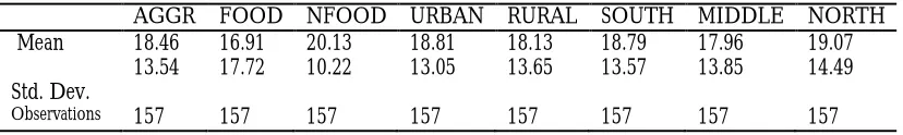
The descriptive statistics in Table 1 show that the inflation series are not different in terms of the average and volatility. On average, inflation is highest in the non-food sector over the period with the food sector recording the lowest average inflation among all the subcomponents considered. The food inflation series happens to be the most volatile while the non-food series is the least volatile among all the subcomponents.
Table 1: Descriptive Statistics
4.2 Time Series Characteristics of the Series in the Dataset
Since the ways the series are modeled depend on their time series characteristics, I investigate the series for their order of integration.
AGGR FOOD NFOOD URBAN RURAL SOUTH MIDDLE NORTH
Mean 18.46 16.91 20.13 18.81 18.13 18.79 17.96 19.07
Std. Dev.
13.54 17.72 10.22 13.05 13.65 13.57 13.85 14.49
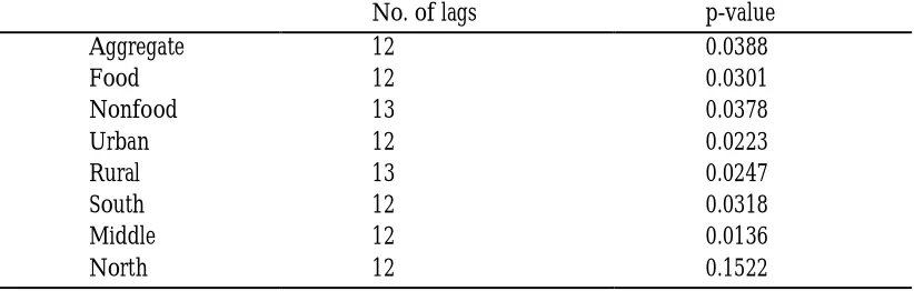
The characteristics of the series are not clear from the visual examination of the graphs in Figure 1, so Augmented Dickey-Fuller (ADF) tests are used to determine whether the series have unit roots. Table 2.2 shows the results of the ADF tests and apart from the north series, all the series are stationary at 5 percent level of significance. This means that the series enter the models at their levels except the north series. Even though the north series is not stationary, including the first difference in the models do not produce any different result from including it at the level. I therefore treat the north series as all the other series and present the results for the levels of all the series. Similarities of the graphs also suggest that their characteristics should not be different.
Figure 1: Graphs of the Level of the Series in the Dataset
0 10 20 30 40 50 60 70
2000 2002 2004 2006 2008 2010 AGGREGATE -20 0 20 40 60 80
2000 2002 2004 2006 2008 2010 FOOD 0 10 20 30 40 50 60
2000 2002 2004 2006 2008 2010 NONFOOD -20 0 20 40 60 80
2000 2002 2004 2006 2008 2010 URBAN -20 0 20 40 60 80
2000 2002 2004 2006 2008 2010 RURAL -20 0 20 40 60 80
2000 2002 2004 2006 2008 2010 SOUTH -20 0 20 40 60 80
2000 2002 2004 2006 2008 2010 MIDDLE 0 20 40 60 80
Table 2: Unit Root Tests of the variables in the Data (ADF p-values)
4.3 Weights
The published weights from Ghana Statistical Service suggests that the weights are constant over the sample period but analysis of the data shows that aggregating the components with the published weights do not produce the same aggregate series as published. I, therefore, compute average post weight for the sample period. The ex-post weights are regression coefficient from the regression of the aggregate series on respective components corrected for serial correlation. These weights are normalized to sum to 1 and the ante weights are the published weights. Table 3 shows the ex-post weights, normalized ex-ex-post weights and the ex-ante weights. A major observation is the reversal of the weights for the rural-urban series, which weights the urban series more that the rural series ex-ante. The normalized ex-post weights are used in calculating the time-varying weights for aggregating the forecasts. The use of these weights as opposed to the ex-ante weights does not change the results significantly enough to change the conclusions.
No. of lags p-value
Aggregate 12 0.0388
Food 12 0.0301
Nonfood 13 0.0378
Urban 12 0.0223
Rural 13 0.0247
South 12 0.0318
Middle 12 0.0136
Table 3: Weights for Aggregating Forecasts
Ex-post Normalized Ex-ante Urban-rural
Urban 0.448850 0.455834 0.535058
Rural 0.535828 0.544166 0.464942
Total 0.984678 1.000000 1.000000
Sectors
Food And Non-Alcoholic Beverages 0.492863 0.492788 0.449084 Alcoholic Beverages, Tobacco and Narcotic 0.046323 0.046316 0.022299 Clothing and Footwear 0.111954 0.111937 0.112855 Housing, Water, Electricity, Gas and Other 0.059017 0.059008 0.069844 Furnishings, Household Equipment and Rou 0.073029 0.073018 0.078266
Health 0.012603 0.012601 0.043276
Transport 0.054722 0.054714 0.062086
Communications 0.004378 0.004377 0.003133
Recreation and Culture 0.031762 0.031757 0.030439
Education 0.006419 0.006418 0.01597
Hotels, Cafés and Restaurants 0.073856 0.073845 0.082825 Miscellaneous Goods and Services 0.033227 0.033222 0.029924
Total 1.000153 1.000000 1.000000
Regions
Western 0.115404 0.115448 0.115603
Central 0.066974 0.066999 0.06953
Greater Accra 0.240317 0.240408 0.242125
Eastern 0.093875 0.09391 0.09248
Volta 0.099928 0.099966 0.102775
Ashanti 0.22458 0.224665 0.223353
BrongAhafo 0.077525 0.077554 0.076107
Northern 0.049047 0.049065 0.048918
Upper 0.031973 0.031985 0.02911
Total 0.999623 1.000000 1.000000
4.4 Granger Causality Tests
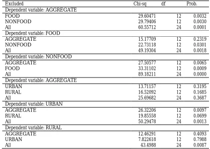
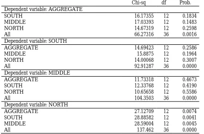
The results from Table 4 show that food and nonfood series Granger-cause the aggregate series individually and jointly and there is a feedback from the aggregate series to nonfood but not to food series. The urban and rural series do not Granger-cause the aggregate series either individually or jointly. The aggregate series, however, Granger-cause the urban series. For the regional series, there is a strong joint Granger causality from the disaggregates to the aggregate series but none from the individual series. Feedback runs from the aggregate only to the north series. These results indicate that the food and nonfood series individually and jointly provide much information in forecasting the aggregate series but the urban and rural series do not provide much information in forecasting the aggregate series as the other disaggregates, either individually or jointly. The joint information contained of the regional series helps forecast the aggregate series but the individual series do not provide enough information to forecast the aggregate series.
Table 4: VAR Granger Causality/Block Exogeneity Wald Test between the aggregate and the disaggregate series
Excluded Chi-sq df Prob.
Dependent variable: AGGREGATE
FOOD 29.60471 12 0.0032
NONFOOD 29.79406 12 0.0030
All 60.55712 24 0.0001
Dependent variable: FOOD
AGGREGATE 15.17709 12 0.2319
NONFOOD 22.73118 12 0.0301
All 49.19304 24 0.0018
Dependent variable: NONFOOD
AGGREGATE 27.50577 12 0.0065
FOOD 33.31102 12 0.0009
All 89.18211 24 0.0000
Dependent variable: AGGREGATE
URBAN 13.71157 12 0.3195
RURAL 16.52092 12 0.1685
All 25.69682 24 0.3687
Dependent variable: URBAN
AGGREGATE 26.32206 12 0.0097
RURAL 19.85558 12 0.0699
All 50.29478 24 0.0013
Dependent variable: RURAL
AGGREGATE 12.46291 12 0.4093
URBAN 7.822618 12 0.7988
Table 4 (Continued): VAR Granger Causality/Block Exogeneity Wald Test between the Aggregate and the Disaggregate Series
Chi-sq df Prob. Dependent variable: AGGREGATE
SOUTH 16.17355 12 0.1834
MIDDLE 17.03393 12 0.1483
NORTH 14.67319 12 0.2598
All 66.27316 36 0.0016
Dependent variable: SOUTH
AGGREGATE 14.69423 12 0.2586
MIDDLE 15.8875 12 0.1964
NORTH 14.00068 12 0.3007
All 92.91287 36 0.0000
Dependent variable: MIDDLE
AGGREGATE 11.73318 12 0.4673
SOUTH 12.33768 12 0.4190
NORTH 10.65658 12 0.5586
All 104.3503 36 0.0000
Dependent variable: NORTH
AGGREGATE 27.12709 12 0.0074
SOUTH 28.88582 12 0.0041
MIDDLE 28.59004 12 0.0045
All 137.462 36 0.0000
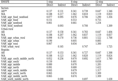
4.5 Results of the Various Models and Model Comparison
For the moving average (MA) models, the direct forecasts are better in all the steps except for the regions where aggregating the forecasts performs better for the 1-step-ahead.
Including additional information from the subcomponents generally performs better for all the models at 1-step-ahead forecasts. The forecasts are, however, less accurate when only food, urban or south series is included in the aggregate model individually, even for the 1-step-ahead forecasts. These results imply that the subcomponents help in producing better short-term forecasts of aggregate inflation if the right subcomponents or their combinations are used in the aggregate model. For the product sector, including the nonfood series improves the forecasts most, while including the rural series improves the forecasts most in the case of the urban-rural classification. In the case of the regional classification, including all the subcomponents improves the forecasts most.
Table 5: Root Mean Square Forecast Error (RMSE) for year-on-Year Inflation*
* Direct forecasts are the forecasts of the aggregate series from a particular model, and the indirect forecasts are the aggregate forecasts that are obtained from aggregating forecasts from the disaggregates
RMSFE 1-step 6-step 12-step
Direct Indirect Direct Indirect Direct Indirect Sectors
AR** 0.137 0.131 0.341 0.739 0.647 1.346
MA 0.188 0.217 1.042 0.810 1.119 0.810
VAR_aggr_food_nonfood 0.077 0.095 0.676 0.706 1.290 1.356
VAR_aggr_food 0.151 0.553 0.755
VAR_aggr_nonfood 0.061 0.661 1.254
VAR_food_nonfood 0.093 0.700 1.309
Urban-rural
AR 0.137 0.158 0.341 0.783 0.647 1.404
MA 0.188 0.207 1.042 0.837 1.119 0.837
VAR_aggr_urban_rural 0.098 0.170 0.736 0.801 1.522 1.708
VAR_aggr_urban 0.190 0.605 0.885
VAR_aggr_rural 0.067 0.654 1.300
VAR_urban_rural 0.165 0.747 1.725
Regions
AR 0.137 0.153 0.341 0.727 0.647 1.308
MA 0.188 0.123 1.042 0.820 1.119 0.824
VAR_aggr_south_middle_north 0.052 0.256 0.670 0.692 1.617 1.760
VAR_aggr_south 0.150 0.491 0.838
VAR_aggr_middle 0.080 0.670 1.285
VAR_aggr_north 0.091 0.680 1.422
VAR_aggr_south_middle 0.065 0.679 1.317
VAR_aggr_south_north 0.065 0.674 1.309
VAR_aggr_middle_north 0.065 0.674 1.309
**The lag length for the AR varies between 1 and 3 that of the MA varies between 1 and 2
5. Conclusions
This study investigates whether forecasting aggregate inflations series by modeling the subcomponents performs better than forecasting the aggregate series directly, and whether including the disaggregate components in the aggregate model improves the forecasts of the aggregate series. The benchmark model with which all the other models are compared is the univariate autoregressive (AR) of the aggregate series. The aggregate series is also modeled using moving average (MA) models. The subcomponents are modeled either independently as autoregressions (AR), moving average (MA) or jointly as vector autoregressions (VARs) with or without the aggregate series.
The results reveal that direct forecasts of aggregate inflation outperform aggregate forecasts that are derived from aggregating forecasts from the subcomponents for all the steps of the forecasts. Including information from the subcomponents improves on the direct forecasts of the aggregate series for 1-step-ahead forecasts. This, however, depends on the subcomponents or their combinations that are used with the aggregate series. A careful selection of the subcomponents into the models is, therefore, needed to achieve more accurate forecasts. The results for 6-step-ahead and 12-6-step-ahead forecasts show that direct univariate forecasts are superior to the forecasts from all the models. This result should therefore be taken carefully because a longer sample is needed to evaluate more independent forecasts errors for these steps.
References
Aron, J. and N. J. Mueller(2008). "Multi-Sector Inflation Forecasting - Quarterly Models for South Africa." CSAE, WPS/2008-27.
Benalal, N.; J. L. Diaz del Hoyo; B. Landau; M. Roma and F. Skudelny(2004). "To Aggregate or Not to Aggregate? Euro Area Inflation Forecasting, ." European Central Bank Working Paper, 374.
Clemen, R. T.(1989). "Combining Forecasts: A Review and Annotated Bibliography." International Journal of Forecasting, 5, pp. 558 - 583.
de Dois Tena, J. ; A. Espasa and G. Pino(2010). "Forecasting Spanish Inflation Using Maximum Disaggregation Level by Sectors and Geographical Regions." International Regional Science Review, 33 (2), 181-204.
Fritzer, F.; G. Moser and J Scharler(2002). "Forecasting Austrian Hicp and Its Components Using Var and Arima Models." Oesterreichische Nationalbank working paper http://www.oenb.co.at/workpaper/pubwork.htm, 73.
Granger, C. W. J.(1969). "Investigating Causal Relations by Econometric Models and Cross-Spectral Methods " Econometrica, 37, pp. 424 - 438.
Grunfeld, Y and Z. Griliches(1960). "Is Aggregation Necessarily Bad?" Review of Economics and Statistics, XLII(1), 1-13.
Hendry , D. F. and K. Hubrisch(2005). " Forecasting Aggregates with Disaggregates." http://www.nuff.ox.ac.uk/users/hendry/HendryHubrich05.pdf, Manuscript.
Hendry , D. F. and K. Hubrisch(2010). "Combining Disaggregate Forecasts or Combining Disaggregate Information to Forecast an Aggregate " European Central Bank Working Paper Peries, No. 1155, pp. 1 - 32
Hendry , D.F and K. Hubrsch(2005). "Forecasting Aggregates with Disaggregates." Manuscript.
Hubrisch, K. (2003). " Forecasting Euro Area Inflation: Does Aggregating Forecasts by Hicp Components Improve Forecast Accuracy? ." European Central Bank Working Paper 247.
Judge, G. G.; W. E. Griffiths; R. C. Hill; H. Lutkepohl and T. C. Lee(1988). Introduction to the Theory and Practice of Econometrics. John Wiley & Sons Inc.
Kohn, J(1982). "When Is Aggregation of a Time Series Efficiently Forecast by Its Past?" Journal of Econometrics, 18(2002), 337-349.
Lutkepohl, H. (1984). "Forecasting Contemporaneously Aggregated Vector Arma Processes." Journal of Business & Economic Statistics, 2(3), 201-214.
Pesaran, M.H.; R.G. Pierse and M.S. Kumar(1989). "Econometric Analysis of Aggregation in the Context of Linear Prediction Models." Econometrica, 57(4), 861-888.
Theil, H(1954). "Linear Aggregationof Economicrelations." Amsterdam: North-Holland. van Garderen, K.J.; K. Lee and M.H. Pesaran(2000). "Cross-Sectional Aggregation of
Non-Linear Models." Journal of Econometrics, 95 (2000), 285-331.