Paper 02-2018-2

(DOI: 10.24874/jsscm.2018.12.02.02)

Mathematical Modelling of Polymer Trajectory During Electrospinning

I. Ferouka1,3,*_{, T. Šušteršič}2,3,4_{, M. Živanović}3 _{and N. Filipović}2,3,4 1 _{Ecole Centrale de Nantes, 1 rue de la Noe, Nantes, France}

2 _{Faculty of Engineering, University of Kragujevac, 6 Sestre Janjic Street, Kragujevac, Serbia} 3 _{Bioengineering Research and Development Center (BioIRC), 6 Prvoslava Stojanovica Street,}

Kragujevac, Serbia

4 _{Steinbeis Advanced Risk Technologies Institute doo Kragujevac, 25 Kneza Milosa Street,}

Kragujevac, Serbia

e-mails: [email protected], [email protected], [email protected], [email protected]

*corresponding author

Abstract

The most important characteristics of the electrospun fibers are their internal morphology and their diameter. They both depend on polymer’s parameters, but also on the process parameters. The motivation for this research is therefore to simulate the jet during electrospinning and analyze the effects of some of the parameters on the jet (and implicitly on fibers), without the necessity to perform the experiments each time. The calculations of the polymer’s behavior between the electrodes was based on the discrete model of Reneker. Thus, the jet was modeled as a system of beads connected by viscoelastic elements. The results were compared to the results obtained in the literature and showed good agreement. The results showed how the jet shape during electrospinning depends on each parameter. The ultimate goal was to establish the exact influence of the above-mentioned parameters on the fibers’ diameter. This would allow to set rough values of electrospinning parameters, which could be further fine-tuned, in order to obtain the fibers with expected characteristics. The beneficial effect of such simulations are time gain, but also reduced material consumption, maintenance costs etc.

Keywords: electrospinning, mathematical modeling, Reneker model, parameters variation

1. Introduction

because of their excellent potential for filtration (Gorji 2017). The applications mentioned above are only part of the various fields that use the mechanical properties of nanofibers.

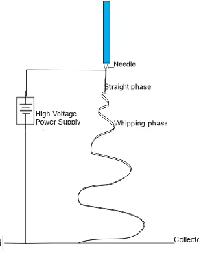
Another advantage is that nanofibers are not difficult to obtain. A typical electrospinning setup only requires a spinneret (syringe pump, syringe and a flat tip needle), a high voltage power supply and a collector plate, which is usually a conductor (Fig. 1).

Fig. 1. Typical electrospinning setup

Initially, the polymer solution is uncharged. As the potential difference is increased, the hemispherical droplet elongates and finally tends to a conical shape known as the Taylor cone. At a particular threshold potential difference, when the forces due to the electric field and the electrostatic repulsion overcome the surface tension forces, jet initiates. First, the jet is straight, but soon it loses stability against transversal distortions and enters a so-called whipping mode. This instability makes the jet loop in spirals with increasing radius (Karra 2007) (Stepanyan 2016). As the jet progresses, it dries, solidifies and is deposited on the collector. Because of the instability of this process, the fibers are most likely to be randomly oriented on the collector (Vught, 2015). However, some researches focused on aligning the fibers from the unstable jet and collecting them in a more structural way. For instance, researchers from Virginia Commonwealth University made experiments based on the idea that with the right speed, the fibers can be collected on the cylinder’s surface and will be aligned in a regular pattern (Huang 2003). Other scientists tried to obtain aligned fibers by employing an auxiliary electrical field (Huang 2003). Further studies have shown that both collector geometry and speed affect the fiber orientation and diameter (Demirtas 2016). Because of the major importance of those characteristics (Stepanyan 2016), many researches have been conducted in order to define exactly which parameters impact on fibers’ internal morphology (orientation, mechanic characteristics, point of break, etc.) and diameter. One example of this is the research by Vong et al. that performed a parametric study to investigate the effects of the pillar morphology (height and thickness) and the electrospinning parameters (applied voltage and working distance) on the overall shape and size of the cone structure, as well as the fiber alignment (Vong 2018).

This is due to the fact that during this phase, the electric field accelerates the jet which leads to a decrease in the jet diameter, by mass conservation. In addition, the electrostatic repulsion between due to excess charges in the solution stretches the jet. This stretching also decreases the jet diameter (Karra 2007).

Several methods have been proposed to measure the fiber’s diameter and to define the exact impact of each parameter on it. Some scientists have tried to establish empirically a formula for the diameter that depends on the flow rate, the dielectric properties of the polymer and the air, the surface tension, the polymer’s viscosity, density and concentration, the current and the voltage

applied. For example, Fridrikh et al. proposed an equation

(

)

2 0 2

* * * 2

* * 2 * 3

Q d

ln

 

 



 − where γ

[N/m] is the surface tension between air and the polymer, Q [m3_{/s] is the flow rate of the solution,}

ε0 [-] is the air dielectric constant, I [A] the total current between the electrodes and χ[-] is the

ratio between the initial length of the filament and the initial jet’s radius (L/R0). However, he

obtained this formula by giving an inconsistently large role to surface tension, which, based on experimental observations, is one of the least important factors in determining fiber diameter

(Gadkari 2014). Helgeson (Gadkari 2014) proposed another formula

(

)

3 2

7 7

0.5

2 0 0

* *

*

* * Q

d c

µ E



 

 

 

 

 

 

 _{   }

−

  _{ } where c [kg/m

3_{] represents the solution’s concentration, μ}

[Pas] is its viscosity, ε [-] the dielectric constant of fluid and E0 [V] the applied electrical field.

This formula gives good solution for PEO water solution, but the main disadvantage is that experimentally it was only verified for one polymer solution.

Other scientists have tried to evaluate the exact influence of only few of the parameters mentioned above on the final diameter. Deitzel et al. (Deitzel 2001) discovered that the morphology of the fibers is strongly dependent on parameters such as the feed rate of the solution, the applied voltage and material parameters, such as concentration, viscosity and surface tension. Some experiments show that the diameter and the gap distance are inversely proportional when the diameter and the feed rate or the viscosity are proportional. Some scientists tried also to evaluate the influence of the applied voltage and calculated numerically the 3D potential field using the Galerkin FEM method and FlexPDE software (Li 2015) but it remains ambiguous (Gadkari 2014).

In order to evaluate the influence of the parameters on the final diameter, today’s researchers work on SEM images of fibers obtained after electrospinning and use Image analyzer software (like DiameterJ, FibraQuant 1.3) to calculate their diameter. MATLAB or JETSPIN (Lauricella, 2016) is often used for calculations, to determine more efficiently and rapidly other characteristics like their length and their orientation but also to create 3D model of electrospinning. For the simulations, Finite Element Method has often been used (Gorji 2017).

viscoelastic jets (Kornev 2011). Some continuum simulations have examined only the steady jet region of the electrospinning jet considering the governing equations pertinent to this regime, namely, the conservation of mass, the conservation of charge, the equation of motion and the electric field balance (Gadkari 2017) (Feng 2003). Another paper by Šušteršič et al. also simulated electrospinning process from the needle to the collector, using commercial ANSYS and their in-house software PAK. They showed that computational approches such as FEM and FVM could be used to implicitly determine the homogeneity of the obtained electrospun fibers based on jet shape during electrospinning (Šušteršič 2018).We chose to base our model on a discrete model of Reneker. We did not find any literature that explained in details a clear, consistent simulation of the polymer jet from the needle to the collector. For example, some models in literature were based on mistaken equations or used coefficients as magic numbers without explaining their meaning. The most complete papers lacked of details especially on how to model the transition between the straight and the whipping phase of the jet. Therefore, our main motivation was to create a detailed and consistent simulation of the polymer jet in between the needle and the collector, compare it to the current state of art and conclude on the influence of some parameters on the electrospun fibers. The paper is organized as following. Second section gives the overview of the governing equations based on Reneker model, that are implemented in Matlab in order to obtain the trajectory or the polymer jet in between the needle and the collector. Third section, Results and Discussion, gives a comparison of the results obtained by other researchers, available in the literature, and our proposed model. Discussion is primarily based on the differences and similarity between the jet trajectories, but also on the obtained fiber diameter collected on the collector.

2. Methods and materials 1.1 Mathematical model

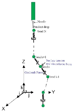
Fig. 2. Schematic of the electrospun fiber model

To describe the movement of the jet, the trajectory of each bead is examined. The position of bead 𝑖 is given by r_i =ix_i+jy_i+kz_i where i, j and k are the unit vectors of the cartesian coordinate system’s axes, x, y, and z.

According to Reneker’s model, the bead is submitted to four forces (Vught 2015; Feng 2002; Karra 2007):

• The Coulomb force, exerted by all the other charged beads and depending on their electrical charge and the distance that separates them from bead i.

(

)

2 3 1

N

i j

ci

j ij

j i

e r r F

l

= 

−

=



Where l_ij =

(

) (

) (

)

• The electric force, derived from the potential difference between the pendant drop and the collector and only applied in the z direction.

0

Ei

eV F

h −

= k (2)

by bead i+ 1, that is defined to be positive and bead i−1, acting in opposite direction, thus negative.

2 1 2 1

, 1 , 1 1, 1,

, 1 1,

F_VEi πa_{i i} σ_{i i} i i πa_{i i} σ_{i i} i i

i i i i

r r r r

l l

+ −

+ + − −

+ −

− −

= − (3)

where

σ is the stress pulling the bead I to bead i+1 or i-1. This stress is characterized by Maxwell’s model of a spring- damper system:

*

d dl G

G

dt l dt µ

 _{= − }

Note: A solution of this DES is proposed in Vugh’s report (Vught 2015)

o ai,i+1 is cross sectional radius of the filament formed by the bead i and i+1

Note: to calculate aij we use the equality settled by the conservation of the

volume a L₀2 =a l2 ,. Here L is assumed to be the initial filament length and set as a length scale.

2 2 0 e L a G



• The surface tension force

( )

( )

(

)

2 2 2

av

sfi i i i i i

i i

a

F K x sign x y sign y

x y



= − +

+ i j (4)

where:

o α represents the surface tension coefficient (N.m-1_{) of the polymer} o K_i 1

R

= is the jet curvature calculated using the coordinates of beads (i-1), i

and (i+1), and the definition of the curvature for three points (Vught 2015)

(

)

(

)

(

)

(

)

(

)(

) (

)(

)

(

)

(

)

(

)

(

)

(

)

(

)(

) (

)(

)

(

)

2 2 2 2 2 2 2 2

1 1 1 1 1 1 1 1

1 1 1 1

2 2 2 2 2 2 2 2

1 1 1 1 1 1

1 1 1 1

.... 2

....

2

i i i i i i i i i i

i

i i i i i i i i

i i i i i i i i i i i i

i

i i i i i i i i

y y x x y y y y x x y y

x

x x y y x x y y

R

x x x x y y x x x x y y

y

x x y y x x y y

− + + + − − + − − + − + + + − − + − − +  − − + − + − − + −   −  +  − − − − −    =  − − + − + − − + −   −   − − − − −    1 2 2                   (5)

and the meaning of “sign” is as follows:

• Sign(x)=1, if x>0 • Sign(x)=-1, if x<0 • Sign(x)=0, if x=0

2 2

i

ci Ei VEi sfi

d r

m F F F F

dt = + + + (6)

And (5) projected on x, y and z leads to the equations of motion for each bead

(

)

(

)

(

)

( )

2 2

, 1 , 1 1 3 , 1 1 , 2 2 2 2 1, 1, 1 2 2 1, 1 * N

i i i i

i j i i

i i

j i j

i _{j i}

i i i i av

i i i i i

i i _{i i}

a e

x x x x

l l d x m dt a a

x x K x sign x

l _{x y}

     + + + + =  − − − −    − + − −      = _{ }   − −    ₊   



(

)

(

)

(

)

( )

, 1 , 1 1 3 , 1 1 , 2 2 2 2 1, 1, 1 2 2 1, 1 * N

i i i i

i j i i

i i

j i j

i j i

i i i i av

i i i i i

i i _{i i}

a e

y y y y

l l d y m dt a a

y y K y sign y

l _{x y}

     + + + + =  − − − −    − + − −      = _{ }   − −    ₊   



(

)

(

)

(

)

, 1 , 1 1 3

, 1

2 1 ,

2

2

1, 1, 0

1 1,

1 *

N

i i i i

i j i i

i i

j i j

i _{j i}

i i i i

i i

i i

a e

z z z z

l l d z m dt a eV z z l h     + + + + =  − − − −    − + −      = _{ }   − − −      



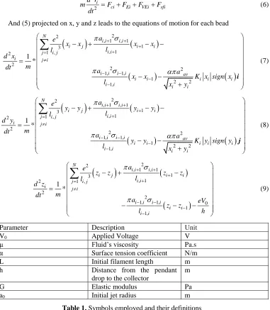
Parameter Description Unit

V0 Applied Voltage V

µ Fluid’s viscosity Pa.s

α Surface tension coefficient N/m

L Initial filament length m

h Distance from the pendant

drop to the collector

m

G Elastic modulus Pa

a0 Initial jet radius m

Table 1. Symbols employed and their definitions

1.2 Simulation of electrospinning on MATLAB

Jet’s trajectory is simulated using the software MATLAB R2017b Differential equations of motion are transformed into a state space notation consisting of first order differential equations that is used as input for MATLAB’s ode45 solver. To do so, all the position velocity and tension coordinates of the system are transformed to a new state vector, called U. Note that the name of U is arbitrary. The size of U depends on the number of beads present in the system.

1.2.1 Differential equation of the stress σ

*

d dl G

G

dt l dt µ

 _

= −

However here we have two time derivatives. We used the method described in Vugh’s report, to solve this equation. The equation is rewritten by moving all time derivatives to one side of the equation. This yields the following equation:

( )

(

)

d G l _G

dt

 _



−

= −

Α new variable,  = −G ln l*

( )

( )

( )

1 2 8 1 2 8

3 3

0

2

* * ln

0

*

0 0 0 0 0 0 0

0

2 2 *

10 0 10 cos 0 0 0 0

103 103

T

i i i N N N

d G G

l dt

U

h i

U u u u u u u

N

i i h i

U Lsin L

N h

H L

 _

 

 

− −

= − −

=

 

= _ _

     

=  _ _ _ _ 

 

=

(10)

Note that in our state vector we will put 𝜎̅ and not σ.

1.2.2 Expression of the state vector

(

)

(

( )

)

(

)

( )

(

)

(

)

, 1 7 , 1 1,1 1

1 1

3

1, , , , 1

2 ₂

, 1 8 , 1 1 1,1 ₁

2 2

, 1 1 3

1 2 3 4 5 6 7 8 , 1 1, ln 1 ln i

i i i i i i i

i j

j N j i i j i i

i i i i i i i _{av i i}

i i i i

i i i i i i i _d i _dt i i i i i i i i i i u

a u G l u u

e

u u

l l

m _{a u G l u u a k u}

l _{u u}

x dx u dt u y u dy u dt u z u dz u dt u   _   + + + =  + + − − + + − _{  + −} − +       + − − − + = ⎯⎯→ =



(

)

(

( )

)

(

)

( )

(

)

(

)

(

)

, 1 7 , 1 1,3 3

3 3

3

1, , , , 1

2 ₂

, 1 8 , 1 3 1,3 ₃

2 2

, 1 _{1 3}

6

2

1 1

3 1, , ,

ln

1

ln

1

i

i i i i i i i

i j

j N j i i j i i

i i i i i i i _{av i i}

i i _{i i}

i

i j

j N j i i j

u

a u G l u u

e

u u

l l

m _{a u G l u u a k u}

l _{u u}

u e u u l m   _ + + + =  + + − − + =                   + −  _{ − +}    _{ }     + −   − −   ₊      −   





(

( )

)

(

)

( )

(

)

(

)

( )

( )

, 1 7 , 1 1,5 5

, 1

2

, 1 8 , 1 5 1,5 ₀

, 1 2

7 , 1

2

8 , 1

ln

ln

ln

ln

i i i i i i i

i i

i i i i i i i

i i

i i i

i i i

a u G l u u

l

a u G l u u _eV

l h G G u l G G u l       + + + + + − − + + −  _{+ −}   _+       + −   − −      − − − ₋ (11)

The whole state vector contains the information of all N beads. It is a column vector and its size is 8xN (N the number of beads). The first 8 lines contain the information (positions, velocities, stresses) for the first bead and then the lines 8x(i-1) to 8xi contain the information for the bead i.

(

)

U= (12)

Based on equations (6), (7), (8) and (9) applied to 𝜎̅𝑖,𝑖+1, and 𝜎̅𝑖−1,𝑖, time derivatives of all the

terms of the state vector are given. Those derivates depend on elements of the state vector. Thus, we can use the ode45 operator of MATLAB to solve the equation and obtain the state vector, and thus the trajectory of each bead.

According to this model, some assumptions have been made concerning the first and the last bead. As the bead i undergoes the forces of bead i+1 and i-1 and for the first bead there is not bead i-1 and for the bead N there is not bead i+1, in the equations of motion of the first bead we consider that every member depending on the hypothetical bead i-1 equals to zero and for the bead N we make the same assumption for every member depending on bead i+1.

1.2.3 Initial conditions

As we mentioned, MATLAB ode45 solver needs an initial condition of the state vector. For the straight jet and according to the paper of Vught, initial state vector is defined as:

0

*

0 0 0 0 0 0 0

T

h i U

N

 

= _ _ (13)

Let us notice that for a straight jet, the curvature of the jet equals to 0. Thus, when we solve the equation in the case of a straight jet, the surface tension force equals to 0.

In case of a whipping jet, it means that its x and y coordinated undergo some perturbation. We decided to take as initial vector:

3 3

0

2 2 *

10 0 10 c

103 os 103 0 0 0 0

T

i i h i

U Lsin L

N

 

− −

     

=      

   

  (14)

For this choice we were inspired by Vught’s paper where the initial vector for whipping phase is taken as follows 1

3 3

0

2

2

*

10

0 10

cos

0

0

0

0

20

20

T

i

i

h i

U

Lsin

L

N





− −













=

_

_

_

_

_

_













General formulas of time and space perturbation have been given in several papers such as:

( )

3

x_i =10− Lcos



( )

h

 

−   −

= _{ }

 

3 2

10 *

i

h z

y Lsin z

h

 

−   −

= _{ }

  (Dasri,

2011) for space perturbation where λ is the wavelength of the perturbation. However, we decided not to use these formulas and fix the perturbation like in Vught’s paper in order not to limit the number of parameters of our study.

Finally, the script has to cope with the introduction of new beads into the system and the removal of beads that have reached the collector There are several ways to do so but we decided to start integration with specified number of beads, which are reintroduced into the system after reaching the collector (Vught 2015). Options of ode45 solver have been used to stop integration when a bead reaches the collector and reintroduce it in the system as a new one.

1.3 Materials

In order to validate our model, we compared our results to those obtained in literature (Table 2). The reason why we focused on papers written by Vught and Dasri is that they also used the Reneker model as basis and used the same initial parameters. We then focused on Karra’s thesis who worked with dimensionless numbers V, FVE, Q and A and examined the influence of some parameters on the jet’s trajectory. Finally, we compared our results to the results of Feng’s review on this subject because he examined the influence of the parameters directly on the fibers’ diameter.

1 _{We take 103 as a denominator in the parenthesis of cos and sin instead of 20 for the matters of}

Reference Initial Values of Parameters Variations

(Vught 2015) V [g1/2_cm1/2_{/s] = 10000 In this review several parameters such} as the number of beads (N), the viscosity (μ), the elastic modulus (G), the surface tension coefficient (α), the initial radius of the jet (a0) and the

applied Voltage between the electrodes (V) have been modified to examine the influence of each parameter on the lateral displacement of the beads on the collector

e [g1/2_cm3/2_{/s] = 8.48} m [g]= 0.283e-5 G [g/cms2_{] = 10}6 h [cm]=20 μ [g/cms]=105 ρ [g/cm3]=1.21e-3 α [g/s2 _]=700 ao [cm]= 150e-4

N number of beads= 20

(Dasri 2011) V [g1/2_cm1/2_{/s] = 500 In this review the parameters mentioned} above were modified to study their influence on the jet’s trajectory. e [g1/2_cm3/2_{/s] = 8.48}

m [g]= 0.283e-5 G [g/cms2_{] = 10}7 h [cm]=20 μ [g/cms]=105 ρ [g/cm3]=1.21e-3 α [g/s2 _]700 ao [cm]= 150e-4 Number of beads=50

(Karra 2007) ₂

0 2

eV mμ V

hLmG

= =100

This review used dimensionless numbers. And varied the surface tension coefficient and the applied Voltage to examine their influence on the jet’s trajectory.

2 2 3 2

e Q

L mG



= =12

2 2 0 2 2

A a

mL G

 

= =9

2 2 0

πa μ F

mLG

VE = =12

h H

L

= = 100

μ [g/cms]=104 _{(1000 kg/ms)} ρ [g/cm3]=1.21e-31000kg/m3 α [g/s2 _]=700

ao [cm]= 150e-4

N number of beads =100

(Zeng 2016) V [g1/2_cm1/2_{/s] = 10000 In this review they examined the} influence of the applied voltage and of the distance from the needle to the collector, on the fibers’ diameter. e [g1/2_cm3/2_{/s] = 8.48}

ρ [g/cm3]=1.21e-3 α [g/s2 _]=700 ao [cm]= 150e-4

N number of beads 20

Table 2. State of art of the influence of some parameters on electrospun polymer jet and nanofibers.

3. Results and discussion

We started by comparing our results with those of Vught (Vught 2015). In his report, the author examined the influence of each parameter on the lateral displacement of the beads on the collector.

He first varied the number of beads from 10 to 100 and observed that the displacement increased with the number of beads (which seems logical). We obtained the same results with our model (Fig. 3 and Fig. 4).

Fig. 3. Jet and displacement of the beads on the collector, N=10

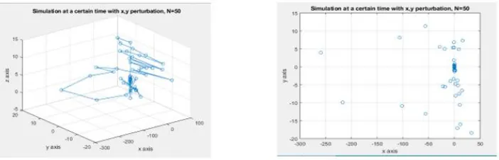
Fig. 4. Jet and displacement of the beads on the collector, N=50.

Then he focused on the effect of the viscosity. He used a system of 10 beads and the initial values of all the other parameters and varied the viscosity. He observed, when he decreased it to 102 _{g/cms (the initial value was 10}6 _{g/cms) and increased it to 10}7 _{g/cms, the result was}

approximately the same. The following figures picture our results that we obtained by implementing the same parameters in our model. (Fig. 5 and Fig. 6)

Fig. 5. Jet and displacement of the beads on the collector, N=10, μ=102

Fig. 6. Jet and displacement of the beads on the collector, N=10, μ=107

On contrary, we observe that with our model even though we increased the viscosity by 105

the lateral displacement of the beads does not seem to vary a lot.

The next parameter that could affect the displacement of the beads, according to our model is the surface tension coefficient. The experiences described in Vught’s paper show that if we increase the coefficient to 900 g/s2 _{(from 700 g/s}2_{) the beads have a slightly smaller displacement}

and if we decrease it to 300 g/s2 _{the displacement becomesslightly larger. The following figures}

Fig. 7. Jet and displacement of the beads on the collector, N=10, α=900

Fig. 8. Jet and displacement of the beads on the collector, N=10, α=300

We almost can not see any remarkable difference which confirms the term “slighly” in Vught’s paper.

Another parameter that could affect the trajectory of the jet is the elastic modulus G. The results in Vught’s paper show that if G is increased to 107 _g/cms2 _{(from 10}6_{) the lateral}

displacement is smaller when if it is decreased to 105 _g/cms2 _{the beads will be more dispersed on}

the collector. In turn we obtain the following results.

Fig. 10. Jet and displacement of the beads on the collector, N=20, G=105

Like in litterature, we observe that the beads tend to form clusters when the elastic modulus is high but that when the elastic modulus is smaller, the beads tend to spread.

Vught examined also the effect of the initial jet radius (when it leaves the needle) on their lateral displacement on the collector. He observed that if the radius is increased to 200e-4 cm (from 150e-4) the lateral displacement is larger and when it is decreased to 100e-4 cm the displacement is smaller. We obtained the following figures (Fig. 11 and Fig. 12) when using the same parameters as Vught and varied the initial jet radius

Fig. 11. Jet and displacement of the beads on the collector, N=10, a0=200e-4 cm

The small number of beads does not allow us to observe a tremendous difference. However, we can say that the beads are a bit more dispersed on the collector when the initial radius is higher

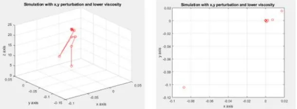
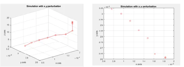
Finally, he wanted to examine the effect of the applied voltage between the needle and the collector. In the paper the results are the following: if the voltage is drastically increased (from 10000 V to 50000 V, meaning 5 times bigger) the displacement of the beads on the collector becomes slightly larger when it undergoes a small decreasing (from 10000 V to 5000 V) the displacement stays approximately the same. We on the other side observe that the more we increase the voltage the more the jet tends to get straight and have a smaller lateral displacement (Fig. 13 and Fig. 14), but according to other studies (Reneker 2000), the length of the straight part of the jet increases when the applied voltage is increased.

Fig. 13. Displacement of the beads on the collector, N=20, V=50kV

Fig. 14. Displacement of the beads on the collector, N=20, V=5kV

We then compared our results to those in the paper of Dasri (Dasri 2011). He used the same initial parameters as in the paper of Vught (Table 2) and varied them in order to examine their impact on the jet’s trajectory.

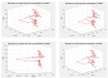
Fig. 15. System of the beads t=0.0004s, N=50, V=500 V (up-left), V=1000 V(up right), V=1500 V (down left) V=2000 V (down right)

He then observed the impact of initial radius and concluded that the lateral displacement of the beads on the collector was larger when the initial radius is increased (from 200e-4 cm to 500e-4cm). When we tried to implement those parameters in our script with 50 beads the program met a problem of integration. However, Dasri obtained the same results as Vught, which we already verified, concerning the influence of the initial radius on the beads’ displacement.

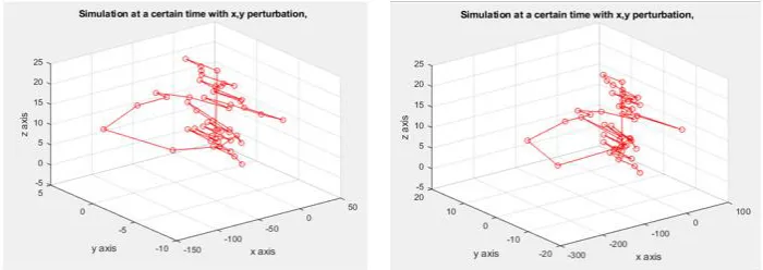
Fig. 16. System of beads, (a) N=20, V=500 V, G=105_{, t=0.0005s, (b) N=20, V=500 V,}

G=107_,t=0.0005s

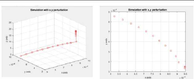
He then examined the influence of the surface tension coefficient of the viscosity on the trajectory. He observed (and we can notice on his figures) that both of those parameters did not have a significant influence on the beads’ trajectory. We may remark that Vught made the same observations. In turn we repeated the experience with the parameters in the paper of Dasri and observed that in fact the trajectory remained approximately the same if we change the surface tension coefficient from 300 g/s2 _{to 900 g/s}2 _{(Fig. 17). We also see (Fig. 18) that the variation of}

the viscosity from 104 _{g/cms to 10}7 _{g/cms does not affect significantly the trajectory either.}

Fig. 17.1 System of beads, N=20, V=500 V, α=300 g/s2 _{(left)- α=900 g/s}2 _{(right), t=0.0005s}

When he examined the effect of the initial radius of the jet he noted that increasing the jet radius to 500e-4 cm leads to a larger area of incoming beads on the collector plate, while decreasing the radius to 200e-4 cm obtains a smaller area. We met some problems of integration when we tried to put an initial radius of 500e-4 cm so we could not compare but this observation confirms the results of Vught.

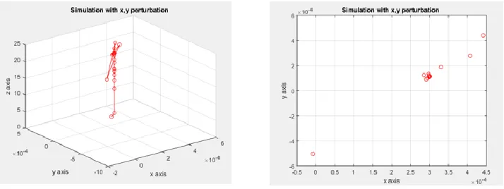
Finally, he examined the influence of the viscosity and observed that using μ=104 _{g/cms or}

μ=107 _{g/cms, the trajectory does not affect the trajectory. We implemented the same parameters}

Fig. 18. System of beads, N=20, V=500 V, a0=100e-4cm,μ=104 g/cms (left)- μ=107g/cms

(right), t=0.0005s

Some literature used dimensionless parameters in order to make the equations dimensionless.

2 0

2

eV μ V

hLmG =

(*) is the dimensionless applied Voltage,

2 2 3 2

e Q

L mG

 =

(**) is the dimensionless

charge,

2 2 0 2 2

απa μ A

mL G =

(***) is the dimensionless surface tension,

2 2 0

πa μ F

mLG VE =

(****) the

dimensionless elastic modulus and

h H

L =

the dimensionless distance between the needle and the collector.

In the thesis of Karra we were given the values of α, μ and a0 which allow us to obtain V0,m,G,h,e that we use in our script out of the values of the dimensionless parameters and L. Actually, let’s name mLG=k (it appears in every group) and put every known variable on one side and every unknown on the other.

From (****) we get that

2 2 0

ve

a k

F

 

=

(*****)

Then (*****) and (***) give us:

2 2 0

απa μ G

ALk

=

(******)

We can now have m=k/LG

From (**) we can now deduce that

2 2 QL kG

e

 =

And we can finally have

2 0 2

VhLmG V

eμ =

The last paper that we used to compare with our results is the report of Zeng (Table 2). In this paper dimensionless parameters and equations are used again but because they don’t give values for α, μ and a0 we could not deduce the values of V0,m,G,h,e. However, they examined the effect of the applied voltage and of the distance from the spinneret to the collector on the fibers’ diameter. In order to make our comparisons, we took the same parameters as in the first two papers (Table 2), varied the applied voltage or the distance between the electrodes as in literature and observed their influence on the radius of the fibers.

In the paper of Zeng, they observed that an increase in the applied voltage from 7.5kV to 17.5kV resulted in a slight increase from 101 to 138 nm and to a slight decrease from 138nm to 123nmwhen the voltage was increased from 17.5 kV to 25kV. The general conclusion is that the applied voltage did not affect a lot the value of the fiber’s diameter. We obtained similar results (Fig. 19) when we used the same initial parameters as in the paper of Vught (Table 2) and increased the applied voltage as in the paper of Zeng (Zeng 2016).

Fig. 19. Radius of the fibers (nm) according to the applied Voltage (V)

Concerning the effect of the distance between the electrodes, they observed that when it was increased from 10cm to 30cm the diameter of the fibers decreased from 134nm to 10nm. We in turn observed a decreasing tendency of the fibers’ diameter when the distance between the electrodes increased (Fig. 20).

Fig. 20. Radius of the fibers (nm) according to the needle-to-collector distance (cm)

Fig. 3 and Fig. 4 confirm the results in Vught’s paper and show that, in an evident way, increasing the number of beads leads to a larger displacement of them on the collector.

Fig. 7, Fig. 8 and Fig. 17 show also that our model validates the observations of Dasri and Vught and that the value of the surface tension coefficient does impacts only slightly the trajectory and the displacement of the beads in a random way.

Fig. 9 and Fig. 10 show that the more we increase the elastic modulus the less the beads will spread on the collector, which confirms the theory of Vught.

Fig. 16. (a) and (b) show, on the other hand, that the elastic modulus influences slightly the trajectory of the beads as noticed Dasri. However, the applied Voltage here was 500 V when in the paper of Vught the applied voltage was 10000 V, which accelerates the beads and could explain the more remarkable effect of the elastic modulus in this paper than in the paper of Dasri.

Fig. 20 confirms the observations that appear in the paper of Feng and show that the fibers’ diameter evolves

Fig. 13 and Fig. 14 show that a higher voltage tends to make the jet straighter and decrease the lateral displacement. Vught on the contrary observed that the applied Voltage did not affect a lot the trajectory.

Fig. 15 shows that the higher the applied voltage is, the more the beads are accelerated, which confirms the theory of Dasri. Fig. 19 confirms the results exposed in the paper of Feng and shows that the value of the applied voltage between the needle and the collector affects only slightly the value of the fibers’ diameter.

In most cases, our model verifies the results of existing simulations, which shows that our model is valid and allows defining the influence of each parameter on the beads trajectory in between the needle and the collector. We have not managed to understand to what are due the problems of integration when they occur but other minor differences could be because we do not use the same method to reintroduce beads in the system or that we do not use the same initial perturbation.

4. Conclusions

We used the discrete model of Reneker to simulate the trajectory of the electrospun polymer from the needle to the collector. The trajectory and the velocities of the system of beads that formed the polymer in this model were calculated according to the second law of Newton and thanks to Matlab solver ode45. This model allowed us to evaluate the influence of some parameters (viscosity, initial radius, surface tension, elastic modulus…) on the trajectory and the displacement of the beads on the collector. Except some problems of integration, most of our results show good agreement with reports from literature. This will allow us in further studies to determine the optimal parameters to obtain optimal fibers without needing to repeat costly experiences. Further studies will also consist in modifying the script in order to obtain a more realistic jet that goes from straight to whipping jet.

Acknowledgements This study was funded by the European Project H2020 PANBioRA [grant number 760921] and grants from the Serbian Ministry of Education, Science and Technological Development [grant number III41007 and grant number OI174028].

References

Deitzel JM (2001). The Effect of Processing Variables on the Morphology of Electrospun Nanofibers and Textiles. Polymer, 261-272.

Demirtas M (2016). Investigation of Collector Geometry and Speed on Orientation, Diameter Distribution and Mechanical Properties of Electrospun Nanofiber. Proceedings of the American Society for Composites: Thirty-First Technical Conference.

Feng (2003). Stretching of a Straight Electrically Charged Viscoelastic Jet. Journal of Non-Newtonian Fluid Mechanics, 116(1), 55-70.

Feng JJ (2002). The Stretching of an Electrified non-Newtonian jet: A Model for Electrospinning.

Physics of fluids, 3912-3926.

Gadkari S (2017, october 12). Influence of Polymer Relaxation Time on the Electrospinning Process: Numerical Investigation. Polymers, 501.

Gadkari SB (2014, Dec 2). Scaling Analysis for Electrospinning. SpringerPlus, 705.

Gorji MJ (2017). Finite Element Modeling of Electrospun Nanofibre Mesh Using Microstructure Archtecture Analysis. Indian Journal of Fibre & Textile Research, 83-88.

Huang ZM (2003). A Review on Polymer Nanofibers by Electrospinning and their Application in Nanocomposites. Composites Science and Technology, 2223-2253.

Feng JJ (2002). Phys. Fluid.

Karra (2007). Modeling Electrospinning Process and a Numerical Scheme Using Lattice Boltzmann Method to Simulate Viscoelastic Fluid Flows. Texas.

Ke ZL (2015). Programming Thermoresponsiveness of NanoVelcro Substrates Enables Effective Purification of Circulating Tumor Cells in Lung Cancer Patients. ACS nano, 62-70.

Kornev KG (2011). Electrospinning: Distribution of Charges in Liquid Jets. Journal of Applied Physics, 124910.

Manea LR A. B.-V. (n.d.). Mathematical Model of the Electrospinning Proces: Effect of the distance between electrodes on the electrospun fibers diameter. Romania.

Lauricella M P.-D.–4 (2016). Three-Dimensional Model for Electrospinning Processes in Controlled Gas Counterflow. The Journal of Physical Chemistry, a, 120(27), 4884–4892. Li YZ (2015). Simulation of Electrostatic Field in Electrospinning of Polymer Nanofibers.

Mathematics of Quantum Technologies, 35-49.

Gorji M R F (2016). Electrospun nanofibers in protective clothing. Elsevier.

Oh B (2013). Nanofiber for cardiovascular tissue engineering. Expert opinion on drug delivery, vol. 10, no 11, p. 1565-1582.

Rafiei SM (2012). Mathematical Modeling In Electrospinning Process Of Nanofibers: A Detailed Review. Cellul Chem Technol, 323-338.

Reneker DH (2000). Bending Instability of Electrically Charged Liquid jets of Polymer Solutions in Electrospinning. Journal of Applied physics, 4531-4547.

Stepanyan RS (2016). Nanofiber Diameter in Electrospinning of Polymer Solutions: Model and Experiment. Polymer, 428-439.

Šušteršič TL (2018). Numerical simulation of electrospinning process in commercial and in-house software PAK. . Materials Research Express, 6(2), 025305.

Vong M (2018). Fabrication of radially aligned electrospun nanofibers in a three-dimensional conical shape. Electrospinning, 2(1), 1-14.

Vught RV (2015). Simulating the Dynamical Behaviour of Electrospinning Processes. Zeng Y, ZP (2016). Numerical Simulation of Whipping Process in Electrospinning. Shanghai. Zhang YL (2005). Recent Development of Polymer Nanofibers for Biomedical and