Classification of Power Signals Using PSO based K-Means Algorithm and Fuzzy C
Means Algorithm
B. Majhi
S. Sabyasachi
S. Mishra
Centurion Institute of Technology
CUTM
Bhubaneswar
India
Abstract
This paper presents a new clustering technique and pattern classification of power signal disturbances using a modified version of S-Transform, which is obtained by taking the Inverse Fourier transform of S-Transform called as modified time-time transform (TT-transform). The TT-transform is a signal processing technique which is used for visual localization, detection, and power signal disturbance pattern classification. The TT-Transform, a new view of localizing the time features of a time series around a particular point on the time axis. TT-Transform has good ability in gathering frequency; it gathers the high frequency signals in diagonal position of the spectrum and suppressing the low frequency signals. The diagonal of TT-Transform represent a simple frequency filtered version of the original signal. The noise can be separated from the effective signal, which can improve the signal-to-noise ratio by using TT-Transform. The extracted features are fed as the input to a Fuzzy C-Means clustering algorithm (FCA) and K-C-Means algorithm for power signal disturbance pattern classification. To improve the pattern classification of the fuzzy C-means and k-means algorithm, the cluster centers are updated using particle swarm optimization technique. Comparison of both the algorithm is made for power signal disturbance pattern classification accuracy
Keywords: FCA, K-Means, power signals, S-Transform, STFT,WT
I.
Introduction
The PQ issues and related phenomena can be attributed to the use of solid-state switching devices, unbalanced and non linear loads, industrial grade rectifiers and inverters, computer and data processing equipments etc., which are being increasingly used in both the industry and home appliances. These devices introduce distortions in the phase, frequency and amplitude of the power system signal thereby deteriorating PQ. Subsequent effects could range from overheating, motor failures, and inoperative protective equipment to power inrush, quasi static harmonic distortions and pulse type current disturbances. Power signal disturbances can also lead to power interruptions, capacitor switching and circuit faults.
Different existing signal processing techniques such as Discrete Fourier Transform (DFT), Short Time Fourier Transform (STFT), Continuous Wavelet Transform (CWT), Discrete Wavelet Transform (DWT), S-Transform etc. are applied to nonstationary power disturbances signals for detection, localization and feature extraction. DFT is an excellent analysis instrument, with a small amount of computations, but for non stationary signals, DFT is insensitive to modifications in time of their spectrum and even to simple time translations. To have time and frequency information simultaneously STFT plays an important role by modulating a fixed window with signal, but fails to give variable resolution.
Wavelet Transform (WT) uses a variable window which gives good frequency resolution and poor time resolution at low frequency and good time resolution and poor frequency resolution at high frequency. However, the Wavelet Transform is sensitive to noise, the WT[8] does not retain the absolute phase information and the visual analysis of the time scale plots that are produced by the Wavelet Transform is intricate. Both the STFT and WT, however, suffer from a trade-off between time and frequency resolutions.
To obtain absolute phase information and improved resolution, S-Transform is used which combines the good features of STFT[2,3] and WT. The properties of S-Transform are that it has a frequency dependent resolution of time-frequency domain and entirely refer to local phase information. S-Transform uses a window which is inversely proportional to the frequency and a Fourier Kernel. The advantage of S-Transform is that it preserves the phase information of the signal, and also provides a variable resolution similar to Wavelet Transform.In case of S-Transform, it uses a Gaussian window and provides variable resolution. S-Transform[6] localizes the real and the imaginary components of the spectrum independently, localizing the phase spectrum as well as the amplitude spectrum. This is referred to as absolutely referenced phase information. But, S-Transform suffers from poor concentration of energy at higher frequency and hence poor frequency localization.
The inverse Fourier transform of the modified S-Transform gives as TT-Transform, which gathers the high frequency signal components in the diagonal position of the spectrum and suppresses the low frequency signal components. Again the TT-Transform is applied to power disturbance signals for feature extraction. The extracted features are fed as input to the PSO based Fuzzy C Means algorithm and PSO based K-Means algorithm for classification. The PSO based K-Means algorithm provides accurate and improved classification results.
This paper presents four sections such as section II presents the derivation of TT-Transform, Section III presents the proposed algorithm and the reference and conclusion is followed by section IV.
II.
TT-Transform
The advantage of S-Transform is that it preserves the phase information of the signal, and also provides a variable resolution similar to wavelet transform. However S-Transform suffers from poor concentration of energy at higher frequency and hence poor frequency localization.TT-Transform, a new view of localizing the time features of a time series around a particular point on the time axis. The TT-Transform [1] is derived from the S-Transform that is inverse Fourier transform of S-Transform.TT-Transform has good ability in gathering frequency; it gathers the high frequency signals in diagonal position of the spectrum and suppressing the low frequency signals. This leads to the idea of filtering on the time–time plane, in addition to the time–frequency plane. Only the diagonal of TT-Transform has been used for signal characterization. The diagonal of TT-Transform represent a simple frequency filtered version of the original signal. The noise can be separated from the effective signal, which can improve the signal-to-noise ratio by using TT-Transform.
The time-frequency analysis of a signal depicts variation of the signal’s spectrum with time. The recently proposed S-Transform is a combination of short-time Fourier transform (STFT) and wavelet transform, since it uses a window inversely proportional to the frequency and a Fourier Kernel.
The standard S-Transform of a signal x(t) is given by a convolution integral [10] as
d
e
e
x
f
t
S
j ft
2 2
) (
.
2
1
)
(
)
,
(
22
(1)
where f is frequency , t and are time variables.
f
1
(2)As the width of the window is dictated by the frequency, it can easily be seen that the window is wider in the time domain at lower frequencies, and narrower at higher frequencies. In other words, the window provides good localization in the frequency domain for low frequencies while providing good localization in time domain for higher frequencies. The disadvantage of the current algorithm is the fact that the window width is always defined as a reciprocal of the frequency.
A significant improvement of S-Transform can be realized by defining the standard deviation of the window as
f k
(3)
resulting in a modified S-Transform as
d
e
e
x
k
f
f
t
S
k j ff t
.
)
(
2
)
,
(
2 2) ( 2 2 2 (4)
Where, and control the width of the window. Choosing k=1, the equation (3.4) can be written as
d
e
e
x
f
f
t
S
j ff t
2 2 ) (
.
)
(
2
)
,
(
2 2 (5)The S-Transform can be written as a convolution of two functions over the variable “t”
f
p
t f
g t f
dtS ,
, ,
(6)Or S
, f
p
t, f
g
, f
(7)Where p
, f
x
ej2f (8)And
22 2 2 , f e f f g
(9)Let B(α, f) be the Fourier transform (from τ to α) of the S-Transform S(τ, f). By the convolution theorem the convolution in the τ (time) domain becomes a multiplication in the α (frequency) domain:
Now defining ) , ( ) , ( ) ,
( f P f G f
B
(10)Where P(α, f) and G(α, f) are the Fourier transform of p(τ, f) and g(τ, f), so we can write 2 2 2 2 ) ( ) ,
( f X f e f
B
(11) Thus S-Transform is the inverse Fourier Transform of the above equation
d
e
e
f
X
f
t
S
f j2
2
.
)
(
)
,
(
2 2 2 (12)and the modified S-Transform is given by
d
e
e
f
X
f
t
S
f j2
2
.
)
(
)
,
(
2 2 2 (13)The TT transform is obtained from the inverse Fourier transform of the modified S-transform as
S t f e df
t
Also inverting the TT -Transform, the original signal x () is obtained as
TT t dt
x(
) ( ,
)Discrete TT-Transform
Let x[ kT], k=0,1,….N-1 denote a time series , corresponding to x(t), with sampling time interval of T. The discrete Fourier transform is given by
1 0 2 ) ( N k N n k j e kT x NT n X (15)As we know the S-Transform is given by
d
e
e
f
X
f
t
S
f j2
2
.
)
(
)
,
(
2 2 2 (16)Using equation (3.16), the S-Transform of a discrete time series x(kT) is given by (letting fn/NT and τ pT where T=1/N
Thus, the discrete TT -Transform is given by
1 0 2 ). , ( ˆ ) , ( ˆ N n N k n j e NT n pT S kT pT T T (17)The discrete TT-Transform contains edge effects since it is obtained from Sˆ . The inversion of TˆT is given by
)
,
(
ˆ
)
(
ˆ
1 0kT
pT
T
T
k
X
N p
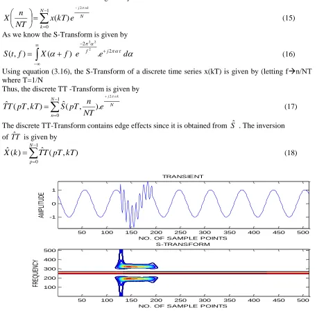
(18)Fig .1 Localization of Transient Signal Using S-Transform
50 100 150 200 250 300 350 400 450 500 -1
0 1
TRANSIENT
NO. OF SAMPLE POINTS
AM PL IT UD E S-TRANSFORM
NO. OF SAMPLE POINTS
FR
EQ
UE
NC
Y
50 100 150 200 250 300 350 400 450 500 100
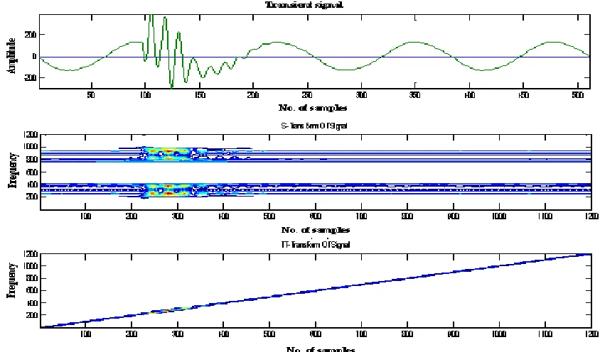
Fig .2 Localization of Transient Signal Using S-Transform and TT-Transform
III.
Proposed Method
(A.)Particle Swarm Optimization is an approach to problems whose solutions can be represented as a point in an n-dimensional solution space. A number of particles are randomly set into motion through this space. At each iteration, they observe the "fitness" of themselves and their neighbours and "emulate" successful neighbours (those whose current position represents a better solution to the problem than theirs) by moving towards them. Various schemes for grouping particles into competing, semi-independent flocks can be used, or all the particles can belong to a single global flock. This extremely simple approach has been surprisingly effective across a variety of problem domains.
PSO was developed by James Kennedy and Russell Eberhart in 1995 after being inspired by the study of bird flocking behaviour by biologist Frank Heppner. It is related to evolution-inspired problem solving techniques such as genetic algorithms. As stated before, PSO simulates the behaviors of bird flocking. Suppose the following scenario: a group of birds are randomly searching food in an area. There is only one piece of food in the area being searched. All the birds do not know where the food is. So what's the best strategy to find the food? The effective one is to follow the bird which is nearest to the food.
PSO learned from the scenario and used it to solve the optimization problems. In PSO, each single solution is a "bird" in the search space. We call it "particle". All of particles have fitness values which are evaluated by the fitness function to be optimized, and have velocities which direct the flying of the particles. The particles fly through the problem space by following the current optimum particles.PSO is initialized with a group of random particles (solutions) and then searches for optima by updating generations. In every iteration, each particle is updated by following two "best" values. The first one is the best solution (fitness) it has achieved so far. (The fitness value is also stored.)
This value is called pbest. Another "best" value that is tracked by the particle swarm optimizer is the best value, obtained so far by any particle in the population. This best value is a global best and called gbest. When a particle takes part of the population as its topological neighbors, the best value is a local best and is called lbest.
PSO is a population based stochastic optimization technique inspired by social behavior of bird flocking.
A concept for optimizing nonlinear functions using particle swarm methodology
1. Each candidate solution is called PARTICLE and represents one individual of a population ( features). 2. The population is set of vectors and is called SWARM(set of feature data points).
3. The particles change their components and move (fly) in a search space. 4. They can evaluate their actual position using the function to be optimized . 5. The function is called FITNESS FUNCTION .
6. Particles also compare themselves to their neighbors and imitate the best of that neighbors .
7. Each particle tries to modify its current position and velocity according to the distance between its current position and pbest, and the distance between its current position and gbest.
So Each particle has
• Individual knowledge pbest
• its own best-so-far position • Social knowledge gbest
• pbest of its best neighbour
Population-based search procedure in which individuals called particles change their position (state) with time.
individual has position --- & individual changes velocity---
Particles fly around in a multidimensional search space.
During flight, each particle adjusts its position according to its own experience.
and according to the experience of a neighboring particle, making use of the best position encountered by itself and its neighbor.
The velocity update equation is given by
and the position update equation is given by
Where “w” is the inertia weight which enhances the exploration ability of particles.
Parameters of PSO
The number of particles :20 –40 particles. In this case 30 particles are considered initially to get good results.
Dimension of particles :It is determined by the problem to be optimized.
Range of particles :It is also determined by the problem to be optimized, we can specify different ranges for different dimension of particles.
Vmax: This is done to help keep the swarm under control. we set the range of the particle as the Vmax.
e.g. X belongs [-10, 10], then Vmax= 20.
One another approach is Vmax= ( UpBound– LoBound)/5
Velocity can be limited to Vmax
Learning/Acceleration factors : c1and c2usually equal to 2. However, other settings were also used in different papers. But usually c1equals to c2and ranges from [0, 4].
The stopping criteria: The maximum number of iterations the PSO execute and the minimum error requirement. PSO Process
1. Initialize particles with random position and velocity vectors. 2. Evaluate fitness for each particle’s position (p).
3. If fitness(p) better than fitness(pbest) then pbest= p . 3. Set best of pbests as gbest .
4. Update particles velocity and position 5. Stop: giving gbest, optimal solution.
6. If not, Go to step 2, and repeat until convergence or a stopping condition is satisfied.
t wv
t cr
pbest
t x t
c r
gbest
t x t
vi 1 i 11 i 2 2 i
t
1
x
t
v
t
1
Inertia weight
For controlling the growth of velocities a dynamically adjusted or constant inertia weight were introduced.
Larger w -greater global search ability
Smaller w -greater local search ability.
By linearly decreasing W-gives best PSO performance
The linearly decreasing inertia weight, ‘w’ is given by
Where k= search number I=maximum number of iteration
Velocity of the particles
Velocity of each particle is updated from the knowledge of the previous velocity and W .
Vmax clamps particles velocities on each dimension and Vmax is saturation point .
Vmax determines “fineness” with which regions are searched
if too high, can fly past optimal solutions
if too low, can get stuck in local minima
The location of each particle is then changed in the next search using its updated velocity information.
The fitness values of all particles are then evaluated and the overall best location is selected.
Constriction Factor
1. Clerc and Kennedy proposed that the constriction factor is effective for the algorithm to converge 2. Constriction factor guarantees the convergence and improves the convergence velocity.
The expression for velocity has been modified as
φ is set to 4.1which gives c1=c2=2.05 and =0.729
PSO algorithm performs well in the early stage, but easily becomes premature in the local optima area.
The velocity is only related with inertia weight and constriction factor.
If the current position of a particle is identical with the global best position and if the current velocity is a small value, the velocity in next iteration will be smaller. Then the particle will be trapped in this area which leads to premature convergence.
(B) Fuzzy C Means Algorithm
In Fuzzy C means clustering [10] we determine the cluster center Ci and the membership matrix U and we thus determine distinct clusters. Fuzzy C Means method is based on minimization of the following objective function: 2 1 1 j i C j m ij N i
m
u
x
c
J
(19)
k
I
w
w
w
k
w
0
1
0
weight
present
w
weight
previous
w
1 0,
4
.
0
,
9
.
0
10
w
w
4
, , 4Where m=2, fuzziness coefficient, uij is the degree of membership of
x
i in cluster j,x
i is thi
thofn
-dimensional measured data, cj is then
-dimensional center of the cluster.
Ck
m
k i
j i
ij N
i m ij N
i
i m ij
j
c
x
c
x
u
u
x
u
c
1
1 2
1 1
,
.
(20)
( C) K-Means Clustering Algorithm
Given a data set of workload samples, a desired number of clusters, k, and a set of k initial starting points, the k-means clustering algorithm finds the desired number of distinct clusters and their centroids [11]. A centroid is defined as the point whose coordinates are obtained by computing the average of each of the coordinates (i.e., feature values) of the points of the jobs assigned to the cluster [12]. Formally, the Fast k-means clustering algorithm follows the following steps.
1. Choose a number of desired clusters, k.
2. Choose k starting points to be used as initial estimates of the cluster centroids. These are the initial starting values.
3. Examine each point (i.e., job) in the workload data set and assign it to the cluster whose centroid is nearest to it.
4. When each point is assigned to a cluster, recalculate the new k centroids.
5. Repeat steps 3 and 4 until no point changes its cluster assignment, or until a maximum number of passes through the data set is performed.
Before the clustering algorithm can be applied, actual data samples (i.e., jobs) are collected from observed workloads. The features that describe each data sample in the workload are required a priori. The values of these features make up a feature vector (Fi1, Fi2, … , FiM), where Fim is the value of the m
th
feature of the ith job. Each job is described by its M features. For example, if job 1 requires 3MB of storage and 20 seconds of CPU time, then (F11, F12) = (3, 20). The feature vector can be thought of as a point in M-dimensional space. Like other
clustering algorithms, k-means requires that a distance metric between points be defined [2]. This distance metric is used in step 3 of the algorithm given above. A common distance metric is the Euclidean distance. Given two sample points, pi and pj, each described by their feature vectors, pi = (Fi1, Fi2, … , FiM) and pj = (Fj1, Fj2, … , FjM),
the distance, dij, between pi and pj is given by:
M
m
ij
F
F
d
im jm1
2
)
(
(21)
If the different features being used in the feature vector have different relative values and ranges, the distance computation may be distorted since features with large absolute values tend to dominate the computation [2]. To mitigate this, it is common for the feature values to be first scaled in order to minimize distortion. There are several different methods that can be used to scale data. The method used in this paper is z-score scaling. Z-score scaling uses the number of standard deviations away from the mean that the data point resides . The z-score equation is
m
m im im
F
F
* (22)
where Fim is the value of the m th
feature of the ith job (i.e., the data point), μm is the mean value of the m th
feature, and σm is the standard deviation of the m
th
feature. Thus, before the algorithm is applied, the original data set is scaled, using the z-score scaling technique, where the feature mean is subtracted from the feature value and then divided by the standard deviation of that feature (i.e., Fim is replaced by its scaled value F
*
im). This technique has
103 The number of clusters to be found, along with the initial starting point values are specified as input parameters to the clustering algorithm. Given the initial starting values, the distance from each (z-scored scaled) sample data point to each initial starting value is found using equation (1). Each data point is then placed in the cluster associated with the nearest starting point. New cluster centroids are calculated after all data points have been assigned to a cluster. Suppose that Cim represents the centroid of the m
th
feature of the ith cluster. Then,
n
F
C
i j jm i im ni
1 * , (23)where F*i,jm is the m th
(scaled) feature value of the jth job assigned to the ith cluster and where ni is the number of
data points in cluster i. The new centroid value is calculated for each feature in each cluster. These new cluster centroids are then treated as the new initial starting values and steps 3-4 of the algorithm are repeated. This continues until no data point changes clusters or until a maximum number of passes through the data set is performed.
PSO Clustering
Using PSO clustering is done and optimal no. of clusters are selected. The center of the cluster are chosen according to Euclidean distance and then refined by the Fuzzy C Means Algorithm.
FCM dynamically determines no. of clusters in the data set.
Let is the swarm of S-particle such that indicates particle ‘i’.
The no. of cluster is given by
Nc =maximum number of clusters Nd= input dimension
And j = 1,…, Nd
And ni is the number of clusters used by the clustering solution represented by the global best particle yˆ such
that
The centers ‘C’ have been randomly initialized as C = (Ci1, Ci2 …Cim).
Initially take the data points and the random centers as the input features.
1. Initialize the swarm S
2. Randomly initialize of each particle ‘i’ in S such that
3. For each particle ‘ ’ randomly choose the centroid to the closest data point using the Euclidean distance.
4. Apply PSO and update velocity and position
5. Update the center by Fuzzy C Means algorithm and K-Means algorithm
6. For each data point the the corresponding center was updated using the formula. where
c k m k i j i ij N i m ij N i i m ij jc
x
c
x
u
u
x
u
c
1 1 2 1 1,
.
ix
xl xi xs
S ,... ,...
Nck ij i
x
n
1 ] 5 , 5 [ ik v iv
ix
NCAnd with K-Means algorithm as
n
F
C
i j
jm i im
ni
1
* ,
7. Repeat until termination criteria are met
8. Repeat step-3 to step-6 for each data point and the optimized center was obtained at the end of iteration. 9. The optimized center was sent as arguments to the Fuzzy C Means algorithm.
10. The Fuzzy C Means algorithm uses the optimized centers obtained as arguments in order to achieve the required clustering.
11. The K-Means algorithm uses the optimized centers obtained as arguments in order to achieve the required clustering and compared with K-Means algorithm.
In the proposed work features such as energy, standard deviation, autocorrelation, mean, variance and normalized values have been extracted from the nonstationary power signals.
The following disturbances have been considered for power signal clustering.
1) Transient
2) Sag with harmonic 3) Swell with harmonic 4) Flicker with harmonic
5) Momentary interruption with harmonic 6) Voltage notch
7) Harmonic 8) Voltage spike 9) Voltage swell
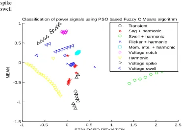
Fig .3: Classification of Power Signals Using PSO based Fuzzy-C Means Algorithm
-1 -0.5 0 0.5 1 1.5 2 2.5
-1.5 -1 -0.5 0 0.5 1
Classification of power signals using PSO based Fuzzy C Means algorithm
M
E
A
N
STANDARD DEVIATION
Transient Sag + harmonic Swell + harmonic Flicker + harmonic Mom. inte. + harmonic Voltage notch
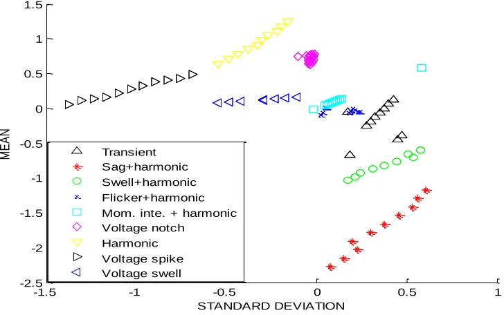
Fig .4: Classification of Power Signals Using PSO Based K- Means algorithm
Fig.3 shows the classification of power signals using PSO based Fuzzy-C Means algorithm and it is found that the power disturbance signals are classified but the cluster pattern visualization is poorer. Fig .4 shows the classification of power signals using PSO based K- Means algorithm and it is found that the power disturbance signals are classified with distinct patterns.
The classification accuracy is shown in the table-1.
Table-1
Sl. No.
Power signal disturbances Accuracy in percentage (%)
PSO-Fuzzy C Means PSO-K-Means
1 Transient 95.66 99
2 Harmonic 93.53 98.45
3 Notch 96.57 97.52
4 Sag 97.48 98.47
5 Spike 96.87 99.48
6 Sag+ Harmonic 93.25 98.67
7 Swell 95.45 97.56
8 Flicker, Sag+ Harmonic 95.87 99.19
% Accuracy 95.58 98.54
From table-2, it is found that PSO K-Means algorithm gives good percentage of accuracy than the PSO-Fuzzy C Means. In both the algorithm in the case of sag ,it is found that the classification accuracy is nearly equal. Moreover the k-means algorithm is preferable for the classification of the power signals.
I.
Conclusion and Reference
The inverse Fourier transform of modified S-Transform is known as TT-Transform, which is applied to extract statistical features and visual localization of power disturbance signals. TT-Transform has potential to localize the power signal waveforms better than the S-Transform as TT-Transform localizes the spectrum diagonally. The extracted features are fed as input to a Fuzzy C Means clustering algorithm (FCA)and K-Means algorithm for pattern classification. To improve the pattern classification a hybrid optimization technique has been applied which is the hybrid of two algorithms such as PSO - Fuzzy C Means and PSO-K means. for comparative assessment of power signal disturbance pattern classification accuracy.
-1.5 -1 -0.5 0 0.5 1
-2.5 -2 -1.5 -1 -0.5 0 0.5 1 1.5
Classification of power signals using PSO based K-Means algorithm
M
E
A
N
STANDARD DEVIATION Transient
Sag+harmonic Swell+harmonic Flicker+harmonic Mom. inte. + harmonic Voltage notch
Particle swarm optimization based K-Means algorithm has achieved higher pattern recognition accuracy in classifying various power signal disturbances than the PSO-Fuzzy C Means classifier. From the simulation results, it is found that the proposed algorithm shows the better classification performance than the existing algorithms in power signal disturbance patterns classification.
References
C. R., Pinnegar, & L. Mansinha, (2203). A method of time-time analysis: The TT-transform. Elsevier Science on Digital Signal Processing, 13(4), 588–603. L. Cohen, “Time-Frequency Analysis”. Prentice-Hall, New Jersey, USA, 1995.
L. Cohen, “Time-Frequency Distributions – A Review”, Proceeding of IEEE, Vol.77, No.7, July 1989, pp.941-981.
E. O. Brigham, “The Fast Fourier Transform And Its Applications”, Prentice-Hall, Englewood Cliffs, New Jersey, 1988.F. S. Chen, “Wavelet Transform In Signal Processing Theory And Applications”, National Defense Publication of China, 1998.
I. Daubachies, “Ten Lectures On Wavelets”, Philadelphia, PA: SIAM, 1992. S. Mallat, “ A Wavelet Tour Of Signal Processing”, London,U.K.:Academic,1998.
Ingrid Daubechies, “The Wavelet Transform, Time–Frequency Localization and Signal Analysis”, IEEE Trans. On Information Theory, Vol.36, No.5, pp.961–1005, 1990.
P. Rakovi, E. Sejdic, L.J. Stankovi and J. Jiang, “Time–Frequency Signal Processing Approaches with Applications to Heart Sound Analysis”, Computers in Cardiology, Vol.33, pp.197–200, 2006.
R. Michael Portnoff, “ Time–Frequency Representation of Digital Signals and Systems Based on Short-Time Fourier Analysis”, IEEE Transactions On Acoustics, Speech, And Signal Processing, Vol.Asp–28, No.1, pp.55–69, 1980.
Wang Y. S., “Sound Quality Estimation for Nonstationary Vehicle Noises Based on Discrete Wavelet Transform”, Journal of Sound and Vibration, Vol.3, pp.1124-1140, 2009.
P.S. Bradley and Usama M. Fayyad: Refining initial points for k-means clustering. In Proceedings Fifteenth International Conference on Machine Learning, pages 91-99, San Francisco, CA, 1998, Morgan Kaufmann.
Khaled Alsabti, Sanjay Ranka and Vineet Singh: An Efficient k-means clustering algorithm. In Proceedings of the First Workshop on High Performance Data Mining, Orlando, FL, March 1998.
P. K., Dash, B. K., Panigrahi, & G. Panda, (2003). Power quality analysis using S-transform. IEEE Transactions on power delivery, 18(2), 406–411.
Dorigo, M., & Gambardella, L. M. (1997). Ant colony system: A cooperative learning approach to the travelling salesman problem. IEEE Transactions on Evolutionary Computation, 1(1), 53–66.
Dash, P. K., Panigrahi, B. K., & Panda, G. (2003). Power quality analysis using S-transform. IEEE Transactions on power delivery, 18(2), 406–411.
Lei Jiang, Wenhui Yang, “ A Modified Fuzzy C-Means Algorithm for Segmentation of Magnetic Resonance Images”, Proc. VIIth Digital Image Computing: Techniques and Applications, Sydney ,10-12 Dec. 2003. B. Biswal, P. K. Dash, S. Mishra, B. Biswal, P.K. Dash, S. Mishra, “A Hybrid Ant Colony Optimization
Technique For Power Signal Pattern Classification”, Elsevier Science, Expert Systems With Applications,Vol.38, No.5, pp.6368-6375, 2011.
R. G., Stock well, L. Mansinha, & R. P Lowe,., (1996). Localization of the complex spectrum: The S-transform. IEEE Transactions on Signal Processing, 44(4), 998–1001
Mohamed N. Ahmed, Sameh M. Yamany et.al, “A Modified Fuzzy C-Means Algorithm For Bias Field Estimation and Segmentation of MRI Data”, IEEE Trans. Med. Imag. Vol.21, No.3,pp.193–199, 2002. C. T. Su, C. F. Chang and J.P. Chiou, “Distribution Network Reconfiguration for loss reduction by Ant Colony
search algorithm”, Electric Power Systems Research, Vol.75, No. 2-3, pp. 190-199, Aug. 2005.
O. J Oyelade, O. O Oladipupo, I. C Obagbuwa, “Application of k-Means Clustering algorithm for prediction of Students’ Academic Performance”International Journal of Computer Science and Information Security,Vol. 7, No. 1, 2010.
H. Timm, C. Borgelt, C. Doring, and R. Kruse, “Fuzzy Cluster Analysis With Cluster Repulsion,” presented at the Euro. Symp. Intelligent Technologies (EUNITE), Tenerife, Spain, 2001.
H. Timm and R. Kruse, “A Modification To Improve Possibilistic Fuzzy Cluster Analysis,” presented at the IEEE Int. Conf. Fuzzy Systems, FUZZ-IEEE’ 2002, Honolulu, HI, 2002.
H. Timm, C. Borgelt, C. Doring, and R. Kruse, “An Extension To Possibilistic Fuzzy Cluster Analysis,” Elsevier Science , Fuzzy Sets Syst., Vol.1, pp. 3–16,2004.
E. E. Gustafson and W. C. Kessel, “Fuzzy Clustering With A Fuzzy Covariance Matrix,” in Proc. IEEE Conf. Decision and Control, San Diego, CA, pp. 761–766, 1979.
D.L. Pham, J.L. Prince, “An Adaptive Fuzzy C-Means Algorithm for Image Segmentation in the Presence of Intensity In homogeneities”. Pattern Recognition Letters.Vol.20,No.1,pp.57–68, 1999.
Mohamed N. Ahmed, Sameh M. Yamany et.al, “A Modified Fuzzy C-Means Algorithm For Bias Field Estimation and Segmentation of MRI Data”, IEEE Trans. Med. Imag. Vol.21, No.3,pp.193–199, 2002. Lei Jiang, Wenhui Yang, “ A Modified Fuzzy C-Means Algorithm for Segmentation of Magnetic Resonance
Images”, Proc. VIIth Digital Image Computing: Techniques and Applications, Sydney ,10-12 Dec. 2003. Math H. J Bollen, Irene Y .H. Gu, Peter G. V. Axelberg, Emmanouil Styvaktakis, “Classification Of Underlying