A Study on Exponentially Weighted Moving Average Control Chart with
Parametric and Nonparametric Approach
Duttadeka, S
Gogoi, B
Department of Statistics
Dibrugarh University
Dibrugarh-786004, Assam
India
Abstract
In this paper, a comparative study of performance of some parametric and nonparametric EWMA control charts for detecting the process mean shift is considered. In section 2, we briefly describe each of the various EWMA models that are taken into account in our present study, Viz. the Parametric
X
-EWMA and Nonparametric Grouped Signed Rank (GSR)-EWMA, for the purpose of comparative study. In Section 3, comparisons of both the procedure are elaborately described. For this, we are using the simulation technique to find out the Average Run Length (ARL) of various EWMA control charts. Results are shown in various tables. Graphs are drawn for easy visual comparison and accordingly, discussions and conclusions are made.Keywords:
EWMA, GSR-EWMA, NEWMA, Parametric and Non-parametric1. Introduction
The Exponentially Weighted Moving Average (EWMA) control charts and other sequential approaches, like Cumulative Sum (CUSUM) charts, are an alternative to Shewhart control charts and are especially effective in detecting small process shifts. Montgomery (2004) observed that the performance of EWMA control chart is approximately equivalent to that of CUSUM chart and in some ways it is easier to set up and operate. Considering this point in view, researchers pay more attention to study and analyze different parametric and nonparametric models of EWMA control chart developed by various scholars in recent times.
A common assumption when evaluating the properties of EWMA charts procedures for controlling the process mean is that the observations are normal with known variance. But generally underlying distribution is not known or hence may not enough information on the variance or shape of the distribution. During the last few years, a new set of EWMA charts have been developed. These are known as Nonparametric EWMA (NEWMA) chart. The properties of this nonparametric rank based procedure do not depend on the distribution of the observations. Rank based procedures are by construction outlier resistant. Some of the works on this line are Bakir and Reynolds (1979), Park and Reynolds (1987), Amin and Searcy (1991), Hackl and Ledolter (1991) , Hackl and Ledolter (1992) etc.
2. Description of Various EWMA Charts
In this section we would briefly highlight the various parametric as well as nonparametric EWMA control chart models that we are considering in this paper for comparison purpose.
2.1. EWMA Control Chart for Individual Observations
Like Shewhart and Cumulative sum (CUSUM) control schemes, a EWMA control scheme (for individual observations) is easy to implement and interpret. For monitoring the process mean, the EWMA control chart consists of plotting
1
(1
)
i i i
Z
X
Z
, 0<
1 … (2.1)Here,
is the weight assigned to the current observation and is called the smoothing constant. Zi is the value of the EWMA after observation i, where the subscript ‘i’ represents the observation number as well as an index of a point in time.The starting value Z0, is often taken to be the target value. The sequentially recorded observations, Xi, can be individually observed values from the process, although they are often sample averages obtained from a designated sampling plan. The process is said to be out of control and action should be taken whenever Zi falls outside the range of the control limits. For additional details concerning EWMA chart are found in Montgomery (2004).
To designing a EWMA control chart, for purposes of process monitoring and detection in shifts, it is necessary to quickly identify optimal EWMA chart parameters. The parameters are optimal in the sense that for a fixed in-control ARL, they produce smallest possible out-of-in-control ARL for a specified shift in the process mean.
Hunter (1986) points out that the EWMA can be thought of as a compromise between the Shewhart
X
and Cumulative Sum (CUSUM) charting procedures. For
=1, the EWMA places all of its weight on the most recent observation, as does theX
chart.For
close to zero, the most recent observation receives little weight, and the EWMA resembles the CUSUM. The choice of
between 0 and 1 determines how much weight the most recent observation will receive.2.2 EWMA Chart for Group of Observations i.e.
X
-EWMA ProcedureThe EWMA control chart is often used with individual measurements. However, if rational subgroups of size
1
n
are taken, then simply replace Xi withX
and
with Xn
. So, in what follows, for EWMA chartfor group of observations, viz,
X
-EWMA, we will assume that the Xi’s are sample means distributed i.i.d 2( ,
)
N
n
with
known.2.3 Description of Nonparametric Grouped Signed Rank (GSR) EWMA Procedure
Grouped Signed Rank (GSR) EWMA is a nonparametric EWMA procedure based on the Wilcoxon-Signed-Rank statistic which was introduced by Wilcoxon (1945). Amin and Searcy (1991) investigate the properties of a nonparametric EWMA (NEWMA) procedure based on the Wilcoxon signed-Rank statistic. They termed this nonparametric EWMA procedure as GSR-EWMA.
Description of the GSR-EWMA Procedure
The GSR-EWMA procedure can be described briefly as follows:
Let(Xt1,Xt2,...Xtg), t = 1, 2, . . . be groups of independent observations taken sequentially, and let
R
t j bethe rank of
X
tj in the group (Xt1, Xt2 ,...Xtg ) for t = 1,2,3,…… and j = 1,2,3,…….,g then
t j t j t j
U
s i g n
X
R
, j = 1,2,.., g ... (2.2)are the Wilcoxon signed ranks of the observations within the tth group of size g. In 1945 Wilcoxon introduced a ranking method that can be used to test the hypothesis that the distribution of the observations is symmetric about some specified value against a class of alternatives that includes symmetric distributions with shifted means. Bakir and Reynolds (1979) applied this idea to the process control problem of detecting departures from a distribution that is symmetric about the control value. They developed and evaluated the properties of a grouped signed rank (GSR)-CUSUM which uses a CUSUM-type stopping rule. The GSR-statistic is given as
1 g
t tj
j
S R
U
… (2.3)The GSR-EWMA procedure similarly accumulates the statistics SRt, t=1,2,… and is based on the statistic
1
(1
)
(
)
t t t
Z
Z
SR
, 0<
<1 … (2.4)where SRt , t=1,2,… represents the signed-rank statistic for the t th
sample of g sequentially recorded observations. The starting value, Z0, is often taken to be the process target value, although other starting value can be used. [Saccucci et. al. (1989)]. The process is considered out -of –control whenever Zt either falls outside the Upper Control limit (UCL) or the Lower Control Limit (LCL). The possible values of SRt are either the even or odd integers between {g (g+1)/2} and {-g (g+1)/2} depending on whether {g(g+1)/2} is odd or even.
Properties of the GSR-EWMA Procedure
The properties of a control chart are determined by the length of time it takes the chart to produce a signal. If the process is in control, then this time should be long so that the rate of false alarms is low, but if the process means shifts, then the time from the shift to the signal should be short so that detection is quick. The number of samples before a signal is usually called the run length, and the expected number of samples is called the Average Run Length (ARL). The ARL is a function of the process mean
. When
0 , the ARL should be large, andwhen
shifts from
0 to
1, the ARL should be small. It should be noted that in order for the GSR procedure tobe able to signal after one group, the maximum allowable UCL is ( 1)
2
g g
, which corresponds to themaximum value that could be computed for Zi when Z0=0. This restriction leads to small in-control ARL values when small group sizes are used unless enhancements are added to the GSR-EWMA procedure such as the fast initial response (FIR) which was introduced by Lucas and Crosier (1982), or adding Shewharts limits to the GSR-EWMA procedure.
3.
Performance comparison of
X -EWMA and GSR-EWMA Control Charts for Monitoring Location
In this section, we compare the performance of two process control procedures for group of observations, viz, the parametric
X
-EWMA and the nonparametric GSR-EWMA. The comparisons of both the procedures are carried out by computing the ARL of the nonparametric and parametric procedure by the simulation technique.Simulation method is used because of the difficulty of computing the ARL values for the GSR-EWMA for various distributions and for different shifts in the process mean / median. Then computer programs have been written to compute ARL values and accordingly evaluate the performance of the control charts to detect different shifts in location under different distributions. For calculation of each ARL value, 5000 runs are repeated. Normal observations are generated using Box-Muller formula (1958) and then necessary values of shift parameters added to each observation to make the process out of control. To generate observations for other distributions, method of inverse integral transformations have used.
Here we have considered four types of distributions viz., Normal (symmetrical sharp-tailed distribution), Uniform (symmetrical light-tailed distribution), Laplace or Double Exponential (symmetrical heavy-tailed distribution) and Cauchy (very long tailed) have been considered since they are different in peakedness or kurtosis. Thus, these distributional forms are selected for two reasons:
(1) They represent a wide range of distributions extending from the short-tailed (Uniform) distribution and the heavy-tailed (Double exponential) distribution.
(2) They are typical for previous literature regarding nonparametric control charts.
The parameters of the distributions are chosen such that all have unit variance. For simplicity, the ARL is calculated under the assumption that the variance of the distribution is known and not estimated.
The control limits for both the control charts, viz.,
X
-EWMA and GSR-EWMA procedures are obtained such that the frequency of the points falling outside the control limits are approximately equal for both the procedures when the processes are in-control. Then the process mean (or median) is shifted by the amount
and the out -of -control ARL values are recorded. The shifts considered in this study are between
=.25 to
=4. The choice ofAnother point which should be noted is that for both the procedures, viz, (parametric)
X
-EWMA and (nonparametric) GSR-EWMA, used in this simulation are based on groups of observations of size g as if we are interested mainly in small shifts, it is preferred to use grouped data; otherwise it is suggested to use the EWMA procedure with ungrouped data. Larger groups sizes allow larger in-control ARL values but can only achieve a minimum out-of-control ARL value of (a larger) g because an entire group must be sampled before a signal. Bakir and Reynolds (1979) concluded that the best group size is somewhere between 5 and 10 depending on the desired value of the in-control ARL and the size of the shift.3.1 Simulation results of ARL Computation
Here, we have displayed some of the results obtained through Simulation method. In the comparison of ARL properties of the GSR-EWMA procedure to
X
-EWMA, it seems natural to match these procedures in the sense that both the charts are considered for group of observations.As already mentioned, using simulation method, we generate observations and calculated ARLs for various choices of chart parameters and shifts in the process mean. The tabulation of ARL s of EWMA charts viz, the parametric
X
-EWMA and the nonparametric GSR-EWMA for various degrees of shift in the underlying process average, positions of the control limits, and magnitudes of the smoothing parameter
are presented in the tables below for Normal as well as Double exponential distribution, Uniform and Cauchy distribution.Table 3.1 (a): Values of the ARL for Two-Sided
X
-EWMA and GSR-EWMA Procedures with g = 6 for Normal i.e. N (0, 1) Data and different
-ValuesTable 3.1 (b): Values of the ARL for Two-Sided
X
-EWMA and GSR-EWMA Procedures with g = 4, 8 and 10 for N (0, 1) Data and
=0.2
0.2
g=4 g=8 g=10
X
-EWMAGSR-EWMA
X
-EWMA
GSR-EWMA
X
-EWMAGSR-EWMA
UCL
SHIFTS( )
0.1735 2.0 0.180 7.2 0.178 11
0.00 18.019 19.0946 39.687 38.743 52.4876 52.528
0.25 4.2484 5.162 4.8776 5.2368 4.8602 5.2904
0.50 1.7476 2.4048 1.776 2.0634 1.7252 2.0718
0.75 0.9028 1.5042 0.8606 1.1854 0.823 1.2688
1.00 0.4542 1.2044 0.3986 0.8142 0.3826 1.0446
1.50 0.1048 1.0176 .047 0.606 0.03 1.0002
0.2
0.4
0.5
X
-EWMA GSR-EWMAX
-EWMA GSR-EWMAX
-EWMA GSR-EWMAUCL SHIFTS( )
0.178 4.2 0.36 8.4 0.453 10.5
0.00 27.533 27.7738 37.9442 38.5574 46.1268 47.7574
0.25 4.677 5.1072 6.3806 7.0572 7.7472 8.9178
0.50 1.7748 2.0698 2.1838 2.6098 2.498 3.3004
0.75 0.8682 1.1496 0.9856 1.3394 1.0708 1.7978
1.00 0.4442 0.7498 0.4756 0.8026 0.4984 1.2562
1.50 0.071 0.3574 0.0738 0.3612 0.0756 1.0194
Explanation of Table 3.1(a) and Table 3.1(b)
The values in Table 3.1(a) gives the ARL values of two-sided
X
-EWMA and GSR-EWMA control charts with group size g = 6 and different
-values for N (0, 1) data . Thus, generating Normal observations, we calculate ARLs for various choices of chart parameters viz., different magnitudes of the smoothing parameter
, such as
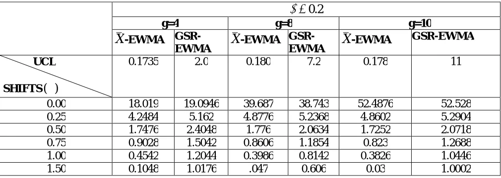
=0.2, 0.4 and 0.5; positions of the control limits in those particular situations, and shifts in the process mean.Table 3.1(b) gives ARL values of two-sided
X
-EWMA and GSR-EWMA control charts with
= 0.2 and different group sizes viz., g = 4,6 and 10 for N (0, 1) data .Graphical Presentation of ARL Values of Normal data
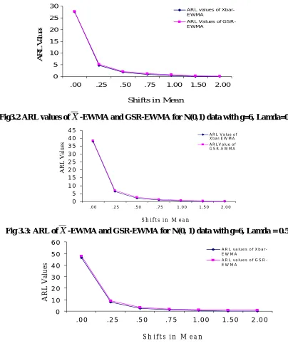
Fig 3.1 ARL values of X -EWMA and GSR-EWMA for N (0, 1) data with g=6, Lamda=0.2
Fig3.2 ARL values ofX -EWMA and GSR-EWMA for N(0,1) data with g=6, Lamda=0.4
Fig 3.3: ARL ofX -EWMA and GSR-EWMA for N(0, 1) data with g=6, Lamda = 0.5
0 5 10 15 20 25 30
.00 .25 .50 .75 1.00 1.50 2.00
Shifts in Mean
A R L V al u es
ARL values of Xbar-EWMA
ARL Values of GSR-EWMA 0 5 1 0 1 5 2 0 2 5 3 0 3 5 4 0 4 5
. 0 0 .2 5 . 5 0 .7 5 1 . 0 0 1 . 5 0 2 . 0 0
S h i f t s i n M e a n
A R L V al u es
A R L V a lu e o f X b a r - E W M A
A R L V a lu e o f G S R - E W M A
0 1 0 2 0 3 0 4 0 5 0 6 0
. 0 0 .2 5 .5 0 .7 5 1 . 0 0 1 . 5 0 2 .0 0
S h i f t s i n M e a n
A R L V al u es
A R L v a l u e s o f X b a r -E W M A
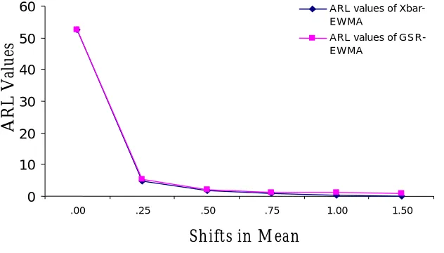
Fig 3.4: ARL values of X-EWMA and GSR-EWMA for N (0, 1) data with g=4 and Lamda=0.2
Fig 3.5: ARL values of X -EWMA and GSR-EWMA for N (0, 1) data with g=8 and Lamda=0.2
Fig 3.6: ARL values of X -EWMA and GSR-EWMA for N (0, 1) data with g=10 and Lamda=0.2
0 5 1 0 1 5 2 0 2 5
.0 0 .2 5 .5 0 .7 5 1 .0 0 1 .5 0
S h i ft s i n m e a n
A
R
L
V
al
u
es
X b a r-E W M A
G S R -E W M A
0 10 20 30 40 50 60
.00 .25 .50 .75 1.00 1.50
Shifts in M ean
A
R
L
V
al
u
es
ARL values of Xbar-EW MA
Table 3.2 (a): Values of the ARL for Two-Sided
X
-EWMA and GSR-EWMA Procedures with g = 6 for Double Exponential Data and Different
-valuesTable 3.2(b): Values of the ARL for Two-sided
X
-EWMA and GSR-EWMA procedures with g = 4, 8 and 10 for Double Exponential Data and
=0.20.2
g=4 g=8 g=10
X
-EWMA GSR-EWMAX
-EWMAGSR-EWMA
X
-EWMAGSR-EWMA
UCL
SHIFTS( )
0.1735 2.0 0.180 7.2 0.178 11
0.00 18.483 18.917 40.2532 38.64 52.8666 51.452
0.25 6.0806 4.6784 4.8538 3.8226 7.7394 5.8888
0.50 2.854 2.119 1.7484 1.5858 2.9532 2.4184
0.75 1.6294 0.9682 0.8468 0.9656 1.5506 1.373
1.00 1.007 0.55778 0.4118 0.6826 0.9128 0.9534
1.50 0.389 0.154 0.0478 0.3904 0.298 0.5016
2.00 0.1364 0.0594 0.002 0.22 0.048 0.2672
2.50 0.039 0.01 0.01 0.11 0.0048 0.0828
3.00 0.0112 0.0004 0.0006 0.0536 0.0006 0.0226
3.50 0.0022 0.0002 0.0002 0.0308 0.0002 0.009
Explanation of Table 3.2(a) and Table 3.2(b)
Table 3.2 (a) gives the ARL values of two-sided
X
-EWMA and GSR-EWMA control charts with group size g = 6 and different
-values for double exponential data. Thus generating Double Exponential observations, we calculate ARLs for various choices of chart parameters viz., different magnitudes of the smoothing parameter
, such as
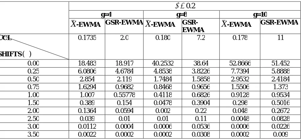
=0.2, 0.4 and 0.5; positions of the control limits in those particular situations, and shifts in the process mean.Table 3.2 (b) gives ARL values of two-sided
X
-EWMA and GSR-EWMA control charts with
=0.2 and different group sizes viz., g=4, 6 and10 for Double Exponential data.0.2
0.4
0.5
X
-EWMAGSR-EWMA
X
-EWMAGSR-EWMA
X
-EWMA GSR-EWMAUCL
SHIFTS( )
0.178 4.2 0.36 8.4 0.453 10.5
0.00 28.1992 27.2028 37.228 37.246 44.2246 46.7838
0.25 6.8814 5.3386 9.8992 7.4578 12.2384 9.1834
0.50 2.9494 2.2786 3.8962 3.0408 4.7094 3.5738
0.75 1.6092 1.2048 1.9616 1.6884 2.2472 1.9394
1.00 0.9788 0.755 1.1042 1.0806 1.2062 1.2174
1.50 0.3576 0.2796 0.3804 0.571 0.397 0.598
2.00 0.0986 0.1206 0.1018 0.184 0.104 0.3532
2.50 0.0188 0.0308 0.0202 0.0898 0.021 0.2266
3.00 0.0046 0.006 0.0046 0.0418 0.0046 0.0418
3.50 0.0004 0.0024 0.0004 0.0172 0.0004 0.0174
Graphical Presentation of ARL Values of Double Exponential data
Fig 3.7: ARL values of X -EWMA and GSR-EWMA for Double Exponential data with g=6, Lamda = 0.2
Fig.3.8: ARL values of X -EWMA and GSR-EWMA for Double Exponential data with g=6, Lamda=0.4
Fig.3.9 ARL values of X -EWMA and GSR-EWMA for Double Exponential data with g=6, Lamda=0.5
Fig. 3.10: ARL Values of X-EWMA and GSR-EWMA for Double Exponential data g=4, Lamda=0.2
. 0 5 1 0 1 5 2 0 2 5 3 0
.0 0 .5 0 1 .0 0 2 .0 0 3 .0 0 4 .0 0
S h i ft s i n M e a n
A R L V al u es
A R L v a lu e s o f X b a r-E W M A
A R L v a lu e s o f G S R -E W M A
0 5 1 0 1 5 2 0 2 5 3 0 3 5 4 0
.0 0 .5 0 1 .0 0 2 .0 0 3 .0 0 4 .0 0
S h ift s in M e an
A R L V al u es
A R L v alu es of X bar-E W M A
A R L v alu es of G S R E W M A
0 1 0 2 0 3 0 4 0 5 0
.0 0 .5 0 1 .5 0 2 .5 0 3 .5 0
S h i ft s i n M e a n
A R L v al u es
A R L V a u es of Xb a r-E W M A
A rl V a lu e s o f G S R -E W M A
0 5 1 0 1 5 2 0
. 0 0 . 5 0 1 . 0 0 2 . 0 0 3 . 0 0
S h i f t s i n M e a n
A R L v al u es
A R L v a l u e s o f X b a r -E W M A
Fig. 3.11: ARL ValuesX-EWMA and GSR-EWMA for Double Exponential data with g=8, Lamda=0.2
Fig. 3.12: ARL ValuesX-EWMA and GSR-EWMA for Double Exponential data with g=10, Lamda=0.2
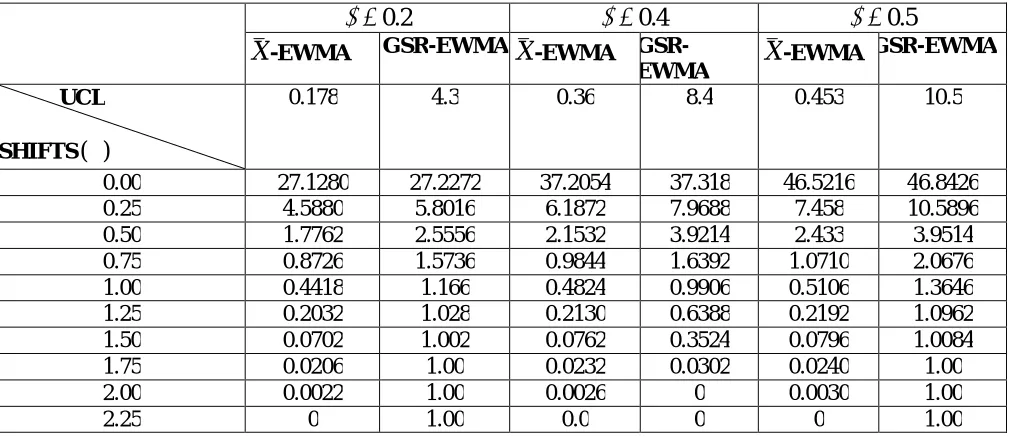
Table 3.3 (a): Values of the ARL for Two-sided
X
-EWMA and GSR-EWMA Procedures with g = 6 for different
-values and Uniform Data0.2
0.4
0.5
X
-EWMA GSR-EWMAX
-EWMAGSR-EWMA
X
-EWMAGSR-EWMA
UCL
SHIFTS( )
0.178 4.3 0.36 8.4 0.453 10.5
0.00 27.1280 27.2272 37.2054 37.318 46.5216 46.8426
0.25 4.5880 5.8016 6.1872 7.9688 7.458 10.5896
0.50 1.7762 2.5556 2.1532 3.9214 2.433 3.9514
0.75 0.8726 1.5736 0.9844 1.6392 1.0710 2.0676
1.00 0.4418 1.166 0.4824 0.9906 0.5106 1.3646
1.25 0.2032 1.028 0.2130 0.6388 0.2192 1.0962
1.50 0.0702 1.002 0.0762 0.3524 0.0796 1.0084
1.75 0.0206 1.00 0.0232 0.0302 0.0240 1.00
2.00 0.0022 1.00 0.0026 0 0.0030 1.00
2.25 0 1.00 0.0 0 0 1.00
0 1 0 2 0 3 0 4 0 5 0 6 0
.0 0 . 5 0 1 .0 0 1 .5 0 2 . 5 0
S h i ft s i n M e a n
A
R
L
V
al
u
es
A R L V a l u e s o f X b a r -E W M A
Table 3.3(b): Values of the ARL for Two-sided
X
-EWMA and GSR-EWMA Procedures with g = 4, 6 and 10 for
=0.2 and Uniform Data0.2
g=4 g=6 g=10
X
-EWMAGSR-EWMA
X
-EWMA
GSR-EWMA
X
-EWMAGSR-EWMA
UCL
SHIFTS( )
0.1735 2.0 0.180 7.2 0.178 11
0.00 17.3468 18.9406 37.2652 37.3488 51.8406 51.02
0.25 4.1784 5.6246 4.7948 5.5866 4.8024 5.7374
0.50 1.7840 2.7526 1.7484 2.3394 1.6908 2.3010
0.75 0.9006 1.7184 0.8486 1.3490 0.7978 1.3660
1.00 0.4910 1.2618 0.4238 0.9308 0.3850 1.0674
1.25 0.2438 1.0702 0.1666 0.7134 0.1294 1.0052
1.50 0.1128 1.0108 0.0488 0.4366 0.0262 1.00
1.75 0.0426 1.00 0.0096 0.0418 0.0032 1.00
2.00 0.0108 1.00 0.0010 1.00 0.0002 1.00
2.25 .0002 1.00 0 1.00 0 1.00
Explanation of Table 3.3 (a) and Table 3.3 (b)
Table 3.3(a) gives the ARL values of two-sided
X
-EWMA and GSR-EWMA control charts with group size g = 6 and different
-values for Uniform data . Thus generating Uniform observations, we calculate ARLs for various choices of chart parameters viz., different magnitudes of the smoothing parameter
, such as
=0.2, 0.4 and 0.5; positions of the control limits in those particular situations, and shifts in the process mean.Table 3.3(b) gives ARL values of two-sided
X
-EWMA and GSR-EWMA control charts with
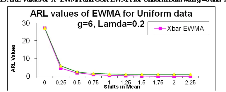
=0.2 and different group sizes viz., g=4,6 and10 for Uniform data.Graphical Presentation of ARL values of Uniform Data
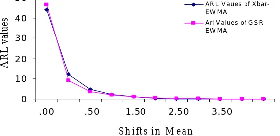
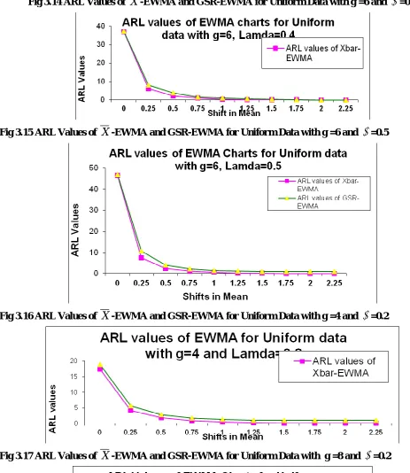
Fig 3.14 ARL Values of X -EWMA and GSR-EWMA for Uniform Data with g =6 and
=0.4Fig 3.15 ARL Values of X -EWMA and GSR-EWMA for Uniform Data with g =6 and
=0.5Fig 3.16 ARL Values of X -EWMA and GSR-EWMA for Uniform Data with g =4 and
=0.2Fig 3.18 ARL Values of X -EWMA and GSR-EWMA for Uniform Data with g =10 and
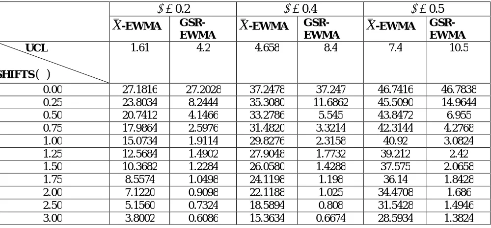
=0.2Table 3.4 (a): Values of the ARL for Two-sided
X
-EWMA and GSR-EWMA Procedures with g = 6 for Cauchy Data and different
-values0.2
0.4
0.5
X
-EWMAGSR-EWMA
X
-EWMA
GSR-EWMA
X
-EWMAGSR-EWMA UCL
SHIFTS( )
1.61 4.2 4.658 8.4 7.4 10.5
0.00 27.1816 27.2028 37.2478 37.247 46.7416 46.7838
0.25 23.8034 8.2444 35.3080 11.6862 45.5090 14.9644
0.50 20.7412 4.1466 33.2786 5.545 43.8472 6.955
0.75 17.9864 2.5976 31.4820 3.3214 42.3144 4.2768
1.00 15.0734 1.9114 29.8276 2.3158 40.92 3.0824
1.25 12.5684 1.4902 27.9048 1.7732 39.212 2.42
1.50 10.3682 1.2284 26.0580 1.4288 37.575 2.0658
1.75 8.5574 1.0498 24.1198 1.198 36.14 1.8428
2.00 7.1220 0.9098 22.1188 1.025 34.4708 1.686
2.50 5.1560 0.7324 18.5894 0.808 31.5428 1.4946
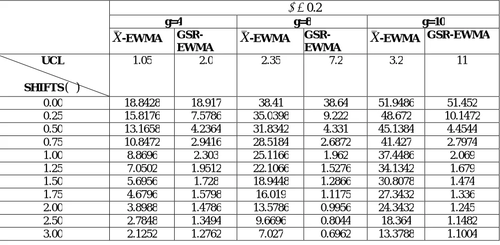
Table 3.4(b): Values of the ARL for Two-sided
X
-EWMA and GSR-EWMA Procedures with g = 4, 8 and 10 for Cauchy Data and
=0.20.2
g=4 g=8 g=10
X
-EWMAGSR-EWMA
X
-EWMA
GSR-EWMA
X
-EWMAGSR-EWMA
UCL
SHIFTS( )
1.05 2.0 2.35 7.2 3.2 11
0.00 18.8428 18.917 38.41 38.64 51.9486 51.452
0.25 15.8176 7.5786 35.0398 9.222 48.672 10.1472
0.50 13.1658 4.2364 31.8342 4.331 45.1384 4.4544
0.75 10.8472 2.9416 28.5184 2.6872 41.427 2.7974
1.00 8.8696 2.303 25.1166 1.962 37.4486 2.069
1.25 7.0502 1.9512 22.1066 1.5276 34.1342 1.679
1.50 5.6956 1.728 18.9448 1.2866 30.8078 1.474
1.75 4.6796 1.5798 16.019 1.1175 27.3432 1.336
2.00 3.8988 1.4786 13.5786 0.9956 24.3432 1.245
2.50 2.7848 1.3494 9.6696 0.8044 18.364 1.1482
3.00 2.1252 1.2762 7.027 0.6962 13.3788 1.1004
Explanation of Table 3.4 (a) and Table 3.4 (b)
Table 3.4(a) gives the ARL values of two-sided
X
-EWMA and GSR-EWMA control charts with group size g = 6 and different
-values for Cauchy data . Thus generating Cauchy observations, we calculate ARLs for various choices of chart parameters viz., different magnitudes of the smoothing parameter
, such as
=0.2, 0.4 and 0.5; positions of the control limits in those particular situations, and shifts in the process mean.Table 3.4(b) gives ARL values of two-sided
X
-EWMA and GSR-EWMA control charts with
=0.2 and different group sizes viz., g=4,6 and10 for Cauchy data.Graphical Presentation of ARL values of Cauchy Data
Fig 3.20 ARL Values of X -EWMA and GSR-EWMA for Cauchy Data with g =6,
=0.4Fig 3.21 ARL Values of X -EWMA and GSR-EWMA for Cauchy Data with g =6 and
=0.5Fig 3.22 ARL Values of X -EWMA and GSR-EWMA for Cauchy Data with
=0.2 and g =4Fig 3.24 ARL Values of X-EWMA and GSR-EWMA for Cauchy Data with
=0.2 and g =103.2. Discussions and Conclusion of Simulation Results
As depicted by Table 3.1(a), for Normal observations, the ARL of
X
-EWMA is slightly less than the GSR-EWMA even though we consider various choices of chart parameter
and shifts in the process mean. It is observed that as the shift in mean increases, the ARL becomes shorter for both the charts.Similarly, from Table 3.1(b), for Normal observations, we have seen that, as we have increased the subgroup sizes, viz, g=4, 6, and 10, for the both charts, the ARL have been increased. Here also the ARL of
X
-EWMA is slightly less than the GSR-EWMA. So, from both the tables, we can conclude that, for Normal observations theX
-EWMA is slightly better than GSR-EWMA chart. The same has been shown graphically by Fig3.1 to Fig 3.6. Thus we may conclude that For a normal distribution which is a symmetrical sharp-tailed distribution, the
X
-EWMA control chart is slightly better than GSR-EWMA chart.Again, as depicted in Table 3.2(a), for Double Exponential observations, the ARL of GSR-EWMA are seems to be less than the
X
-EWMA even though we consider various choices of chart parameter
and shifts in the process mean. Moreover, as the shift in mean increases, the ARL becomes shorter for both the charts.Similarly, from Table 3.2(b), for, Double Exponential observations, we have seen that, as the group sizes increases, viz, g=4, 6, and 10, for the both charts, the ARL have increased. Here also, ARL of GSR-EWMA is found to be less than the
X
-EWMA.So, from both the Tables 3.2(a) and 3.2(b) and Figures 3.7 to 3.12, it may be concluded that, for the Double Exponential observations, the performance of GSR-EWMA is slightly better than
X
-EWMA chart. For Double Exponential distribution, the GSR-EWMA control chart performs slightly better than
X
-EWMA chart, so GSR-EWMA may be preferred under this distribution.Again, as depicted in Table 3.3(a), for Uniform observations, the ARL of
X
-EWMA are seems to be less than the GSR-EWMA even though we consider various choices of chart parameter
and shifts in the process mean. Moreover, as the values of
increases, ARL value increases and as the shift in mean increases, the ARL decreases for both the charts.Similarly, from Table 3.3(b), for Uniform observations, we have seen that, as the group sizes increases, viz, g=4, 6, and 10, for the both charts, the ARL have increased for a fixed
=0.2. Here also, ARL ofX
-EWMA is found to be less than the GSR-EWMA.So, from both the Tables 3.3(a) and 3.3(b) and Figures 3.13 to 3.18, it may be concluded that, for Uniform observations, the performance of
X
-EWMA is comparatively better than GSR-EWMA chart.Table 3.4(a) depicts that for Cauchy observations, the ARL of GSR-EWMA are seems to be less than the
X
-EWMA when we consider various choices of chart parameter
and shifts in the process mean. As shift in mean occurs, the ARL of GSR-EWMA chart becomes shorter as compared toX
-EWMA chart. Moreover, as the shift in mean increases, the ARL decreases for both the charts.Similarly, from Table 3.4(b), for, Cauchy observations, we have seen that, as the group sizes increases, viz, g=4, 6, and 10, for the both charts, the ARL have increased. Here also, ARL of GSR-EWMA is found to be less than the
X
-EWMA.So, from both the Tables 3.4(a) and 3.4(b) and Figures 3.19 to 3.24, it may be concluded that, for the Cauchy observations, the performance of GSR-EWMA is better than
X
-EWMA chart. The GSR-EWMA control chart may be recommended for the Cauchy distribution.
References
Amin, R.W. and Searcy, A.J. (1991): A Nonparametric Exponentially Weighted Moving Average Control Scheme, Commun. Statist.-simula., 20(4), 1049-1072.
Bakir, S.T. and Reynolds, M.R. Jr. (1979): A nonparametric procedure for process control based on within-group ranking, Technometrics, vol21, 175-183.
Box, G.E.P and Muller, M.E. (1958): A Note on the Generation of Random Normal Deviates, The Annals of Math.Statist., vol. 29, 610-611.
Hackl, P. and Ledolter, J. (1991): A control chart based on ranks, Journal of Qual. Tech.,Vol 23, 117-124. Hackl, P. and Ledolter, J. (1992): A New nonparametric Quality Control Technique,Commun. Statist. -Simula.,
21(2), 423-443.
Hunter, J.S. (1986): The Exponentially Weighted Moving Average, Journal of QualityTechnology 18, 203-210. Lucas, J.M. and Crosier, R.B. (1982): Combined Shewhart-CUSUM Quality Control Schemes, Jrnl.Qual. Tech,
14, 51-59.
Montgomery, D. C. (2004): Introduction to Statistical Quality Control, 4th Edition John Wiley Sons – New York. Park, C and Reynolds, M.R. (1987): Nonparametric procedures for monitoring a Location parameter based on linear placement statistic, Sequential Analysis 6(4), 303-323.
Roberts, S.W. (1959): Control Chart Tests Based on Geometric Moving Average, Techometrics, vol.3, 239-250. Saccucci, M.S., Amin, R.W., and Lucas, J.M. (1989): EWMA control Schemes with VSI, Drexel University Faculty Working Paper Series, WPS-5.