INTRODUCTION
In the Russian Federation, approximately 40 to 68 major floods occur each year. The largest floods occurred in 2012 in Krasnodar Territory and in the Republic of Adygea in 2017.
The need to protect the rapidly developing Russia’s economy and population requires timely warnings based on reliable forecasts. While such warnings should be issued for about one of ap-proximately 2.6 million Russian streams (most of which are ungauged or poorly gauged), this can be done only in fully automated and quite ap-proximate (virtually, qualitative) mode. In chang-ing climate and variable anthropogenic impact on river basins, as well as due to quite low density of the surface hydrometeorological network, flash flood forecasting based on “traditional”
physical-ly based, or conceptual, or statistical hydrologi-cal models often becomes inefficient [Pivovarova 2016]. Thus, the basic task of the presented study can be posed as developing a fully automated system of qualitative forecasting risks of flooding regardless of the quality and spatiotemporal reso-lution of the available hydrometeorological data.
The authors of the presented study realize that accurate and timely flash floods forecasting, espe-cially, in ungauged and poorly gauged basins, is one of the most important and challenging prob-lems to be solved by the international hydrologi-cal community; also, they understand that the ac-curacy and efficiency of forecasting depend, first of all, on 1 – data resolution and quality and 2 – the ability of used models to reflect the runoff generation processes properly. Therefore, the effi-ciency of flood forecasting in different basins also
Published: 2018.01.01 Volume 19, Issue 1, January 2018, pages 177–185
https://doi.org/10.12911/22998993/79419
Use of MLCM3 Software for Flash Flood Modeling and Forecasting
Daria Sokolova
1, Vadim Kuzmin
2, Artur Batyrov
1, Inna Pivovarova
3*,
Ngoc Anh Tran
4, DinhKha Dang
4, Kirill V. Shemanaev
11 Russian State Hydrometeorological University, Malookhtinsky 98, Saint Petersburg 195196, Russia, e-mail:
2 Russian State Geological Prospecting University, Miklouho-Maklay’s St. 23, Moscow 17997, Russia, e-mail:
3 Saint-Petersburg Mining University, 2, 21 Line, Vasilievsky Island, Saint Petersburg, 199026, Russia
4 VNU University of Science, Vietnam National University (VNU), 334 Nguyen Trai, Thanh Xuan, Hanoi, Vietnam,
e-mail: [email protected]
* Corresponding author's e-mail: [email protected]
ABSTRACT
Accurate and timely flash floods forecasting, especially, in ungauged and poorly gauged basins, is one of the most important and challenging problems to be solved by the international hydrological community. In changing climate and variable anthropogenic impact on river basins, as well as due to low density of surface hydrometeorological network, flash flood forecasting based on “traditional” physically based, or conceptual, or statistical hydrological models often becomes inefficient. Unfortunately, most of river basins in Russia are poorly gauged or ungauged; besides, lack of hydrogeological data is quite typical. However, the developing economy and population safety necessitate issuing warnings based on reliable forecasts. For this purpose, a new hydrological model, MLCM3 (Multi-Layer Conceptual Model, 3rd generation) has been developed in the Russian State Hydrometeorological
University. The model showed good results in more than 50 tested basins.
will be different, but, while we are keen on pre-dicting the overall risk of flooding (say, in terms of its probability and level of danger), we agree, by default, that the streamflow forecasting carried out for a big number of streams cannot be as ac-curate as that for a single stream, and should sup-pose presenting forecasts in the same format (for instance, the flood risk level.
The hydrological models that would be suit-able for implementation in automated mode should be:
• easily, fast and efficiently calibrated (and re-calibrated, if necessary);
• inexpensive in terms of computational/proces-sor resources [Phong et all. 2015];
• forced by commonly available data (such as precipitation and evaporation/evapotranspira-tion), and
• reliable enough even when being forced by “bad” data.
For this purpose, a new hydrological model, MLCM3 (Multi-Layer Conceptual Model, 3rd
generation) has been developed in the Russian State Hydrometeorological University.
It should be noted that a large part of hydro-logical studies, monographs and articles are de-voted to hydrological modeling, as well as the development of new hydrological models and the improvement of the existing ones.
The article [Kuzmin 2009] initiates a series of three articles on the automatic calibration of op -erational multi-parameter models used for flash flood forecasting in an automated regime. The first article of the series contains a critical anal -ysis of the “mainstream“ in hydrological mod -els calibration and presents the basic principles of the Stepwise Line Search (SLS) algorithm and its modifications, practically feasible and robust parametrization approaches that would be suitable for an automated systems used for flash flood forecasting.
In the work [Alfonso 2010] written by lead-ing European experts in the field of flood and flash flood modeling, the latest studies of the ef-fectiveness of optimizations of various versions of lumped, distributed and half-distributed hydro-logical models, are summarized. In the Russian Federation, conclusions made in this paper can be used as a methodological basis for the devel-opment of models in basins with a low spatial-temporal discreteness of ground-based obser-vations, so individual ideas of the article were
used in developing the calibration method for the MLCM3 model.
It is known that the models used by the fore-casting organizations should be both reliable and simple, but also be able to provide sufficient lead-time for warnings and the desired degree of accu-racy. In general, the choice of the model depends on the following factors: the amount of data avail-able, the complexity of the hydrological processes to be modeled, the reliability required, the accura-cy and lead-time, the type and frequenaccura-cy of flood-ing, and user requirements [Refsgaard 1997] .
In many cases, for hydrological modeling and forecasting, when projections of expenditure or water levels along the river are needed, hydrome-teorology specialists use the models of “rainfall-runoff” type in conjunction with the models of the propagation of the flood wave. If the precipita-tion is presented in the form of snow, snowmelt models are used. These models differ in terms of accuracy and complexity, occupying the en-tire spectrum from the models based on the use of the index of previous humidification, to mul-tiparameter conceptual models or process models [WMO. Guide to Hydrological Practices 1994].
In our case study, in which we had to find a certain compromise between various extremes, conceptual models seem to be preferable. Typi-cally, the conceptual, hydrological models in-clude the description of the processes of water supply, loss, redistribution of moisture in the soil, surface, soil and subterranean inflow to the chan-nel network, as well as their transformation into the hydrograph. However, the degree of detail in the description of these processes, as well as the dependencies used in various models, can vary significantly and lead to their diversity.
This type of models is operationally imple-mented in many countries. For example, the Hy-drologiskaByrånsVattenbalansavdelning model (HBV) was developed by Bergström at the Swed-ish Meteorological and Hydrological Institute for modeling and analysis of river runoff. The HBV model is a conceptual model that converts pre-cipitation, atmospherical temperature and poten-tial natural water loss into either snow melting, or into runoff or inflow into the reservoir. The HBV model can be considered as a model with half-distributed parameters: the catchment area is di-vided into private catchments, and the altitudinal zoning method is also applied [Johansson 1997].
research group IPH-UFRGS, which specializes in large-scale hydrology. This model is used to work with many South American basins. MGB-IPH is a sediment-drain model that uses precipitation, air temperature, relative humidity, wind speed, insolation and atmospheric pressure to calculate the flow rate in a given basin.
The well-known Sacramento Soil Moisture Accounting Model (SAC-SMA) [Burnash et al.1973, Reed et al. 2005] is successfully im-plemented in the United States for flash flood forecasting for four decades. This model is very popular among hydrologists. The original version of the Sacramento model includes 16 optimized parameters, the values of which can be estimated by observing soil moisture and entering data on soil type; however, in most cases, it is possible to replace 5–7 parameters with constants without any modeling quality loss.
FEATURES OF THE CONCEPTUAL
HYDROLOGICAL MODEL MLCM3
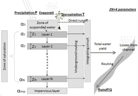
In this paper, a basic version of the MLCM3 is presented. MLCM3 is a rainfall-runoff model with a flexible structure and high level of “con-ceptualization”. The model forcing includes pre-cipitation and evaporation data, basically coming from NWP model output. Water comes to the out-let through several layers; their number, as well as two parameters (thickness and infiltration rate) for each of them, surface flow velocity (when the top layer is full of water) are optimized.
MLCM3 has a variable number of parame-ters: a number of layers N, depth of ith layer Z
i,
in-filtration rates αi (which can be constant or
com-puted using individual equations for each layer), and velocity of the surface runoff α0. Thus, a total number of parameters will be equal to 2N + 2. If the unit hydrograph is approximated with 2-pa-rameter Gamma-distribution, two extra parame-ters are added. Furthermore, Muskingum-Cunge, or kinematic wave, or any other routing scheme can be applied; in our case, Muskingum-Cunge algorithm is used by default. The Muskingum routing procedure relies on the use of the storage-outflow relationship
Q
2=
C
1I
1+
C
2I
2+
C
3Q
1, where Qj is the outflow rate; Ik is the inflow rates coming from upstream; coefficients C1, C2 and C3 depend on the Muskingum parameters X and K that may be optimized or treated as empirical and fitted when an outflow hydrograph is available ata gauge. A priori estimates of X and K can be also obtained by using the physical channel properties
x, c, b and s. Figure 1 shows the scheme of the conceptual hydrological model MLCM3 and the Table 1 present the forcing data for it [Barrett 2008, Kuzmin et al. 2008].
All the parameters can be optimized; there are many possible strategies to use the available pro-cessor resources for this purpose. For instance, for urban catchments, a number of layers can be fixed (up to 2), and all possible parameter sets can be examined. If some moisture holding data are available, a certain number of parameters can be also fixed, while the rest of them will be opti-mized. Alternatively, soil moisture content of the top layer can be determined by using the satel-lite observations (e.g. soil moisture data from the AMSR-E), while the rest of layers will be param-eterized separately, etc.
Time step may also vary. There are two de-fault options (1 h and 24 h), but a modeler can set any value depending on his/her needs.
INTER-COMPARISON OF THE MLCM3
MODEL WITH THE SACRAMENTO MODEL
The conceptual hydrological model of the Sacramento Soil Moisture Accounting Model (SAC-SMA) is one of the most well-known and most commonly used hydrological models in modeling and forecasting. Only the standard hydrometeorological network observations, cli-matological information and publicly available cartographic data are used as the “input”. How-ever, such a hydrological model is extremely difficult to calibrate if there is insufficient mea-surement data (shortage of posts and lack of measurement of some quantities are a fact in the Russian Federation).
Inter-comparison of MLCM3 and SAC-SMA demonstrated their similar efficiency in the flash flood modeling based on the radar precipitation data. However, unlike SAC-SMA, MLCM3 was calibrated by using SCE algorithm and imple-mented without soil data. The obtained results for test catchments are presented in Table 2.
by 5 storages and MLCM has a higher level of conceptualization, than SMA. Unlike SAC-SMA, it does not require any soil data (however, it can be used if such data are available).
The main advantage of the MLCM3 model is its ability to use it with a smaller amount of input information than is required in the case of the Sacramento model. The main features of the MLCM3 model, in contrast to the Sacramento model, are its high predictive efficiency and the performance of calibration and validation proce-dures in a fully automated mode.
MLCM3 SOFTWARE FOR FLASH FLOOD
FORECASTING
The software «MLCM3» is intended for forecasting and modeling rainfall flash floods. The MLCM3 is an application that utilizes an intuitive user interface that makes imputing and editing experiments with data fast and efficient. This program uses a client/server based model. The client is what the user uses to add research-er’s records as well as edit them. The client pro-gram will communicate with a university server
(RSHU) that saves all the information for each researcher (information about experiment results) and includes some of their personal information (login and password).
The main function of the MLCM3 software is the processing of input files containing data on hydrometeorological variables at the time of the calculation. As a background forecast, the data of the external mesoscale meteorological model (Weather Research and Forecasting (WRF) – a package of modeling meteorological processes) are used. The program is designed for forecast-ing the river flow, which allows assessforecast-ing the hydrometeorological risks in the conditions of climate change and variable anthropogenic load on river basins.
Figure 1. The conceptual hydrological model MLCM3
Table 1 Forcing data for MLCM3
Data type Symbol
Precipitation P
Evapotranspiration ET
Catchment area S
Main channel length L
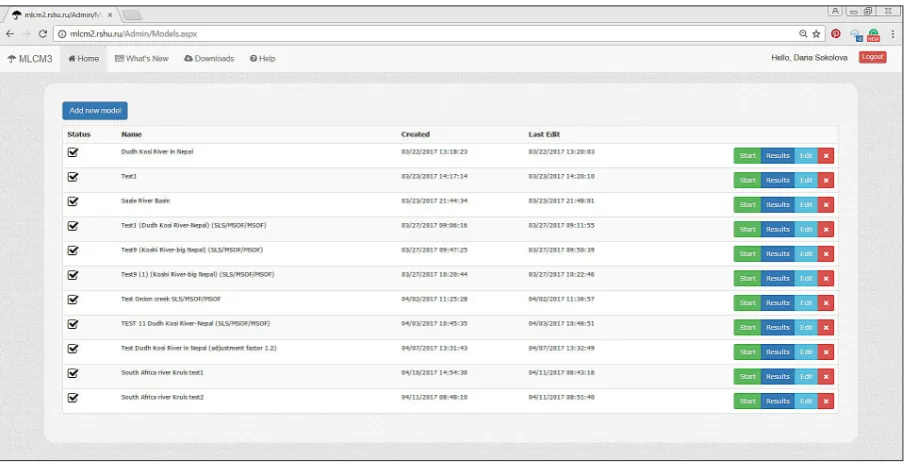
There are two different types of users: Admin Users and Users. Admin Users are MLCM3 soft-ware developers who have the authority to give Users the access to use the software. On the other hand, users have the right to work with the soft-ware and upload information to it. In order to get started with the software, one needs to go to the site http://mlcm2.rshu.ru/ and log in to their ac-count with the login and password received in ad-vance from the administrator. The Figure 2 shows the interface of the MLCM3 software.
The top tabs are optional and include: • In the tab “Home” – store experiments. • In the tab “What`s New” – read information
about the program’s improvements.
• In the tab “Downloads” – download a con-verter for data sets.
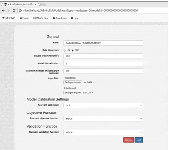
• In the tab “Help” – download User’s Manual. In MLCM3, it is possible to carry out a full technical adjustment of the model parameters.
One can choose from three types of calibration and pre-calibration. The user can perform the SLS calibration (Stepwise Line Search), the Nelder-Mead methods and the extended Nelder-Nelder-Mead. Furthermore, the user can select the type of the objective function and the validation. The choice includes: the root-mean-square error, the crite-rion S/σ and the multi-scale objective function MSOF. In order to emulate this multi-scale nature of manual calibration, we employ an objective function composed of contributions from a wide range of time scales of aggregation. The particular objective function MSOF used in this work was proposed by Koren and has the following form:
( )
(
)
∑
∑
= =
−
= mk
i oki ski
k k
X q q J
1
2
, , , , n
1
2
1
σ
σ
where: qo,k,iand qs,k,i – measured and modeled
discharge of water averaged over the time interval k
Table 2. The results of numerical experiments on modeling of rainfall flash floods
No. Basin Watercourse code Value of the objective function MSOF
MLCM3 SAC-SMA
1 Austin – Onion Creek 08159000 18.87 19.36
2 Justin – Denton Creek 08053500 14.72 16.13
3 Houston – Greens Bayou 08076000 11.03 11.35
4 Georgetown – South Fork San Gabriel 08104900 14.80 16.22
5 Greenville – Cowleech Creek 08017200 13.70 14.39
6 Houston – Brays Bayou 08075000 25.65 27.02
7 Hunt – Guadalupe River 08165500 28.91 30.99
8 Justiceburg – Double Mt Fork 08079600 11.95 12.19
σk – Mean square error deviation of the
discharge of water rate of k n– Total number of scales,
mk – the number of items of each scale k
where qo,k,i and qs,k,i k, are the observed and simulated flows averaged over time interval k ; σk is the standard deviation of
discharge at that scale; n is the total num-ber of scales used, and mk is the number of ordinates at the scale k .
This weighting scheme assumes that the un-certainty in modeled streamflow at each scale is proportional to the variability of the observed flow at that scale. Another important advantage of using the multi-scale objective function (MSOF) is that it smoothes the objective function’s sur-face, and, hence, reduces the likelihood of the search getting stuck in tiny “pits”.
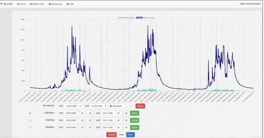
In Figure 4, tabs are provided for the map-ping of a single stream. All buttons are optional and simulation, calibration and validation peri-ods can be set manually in cells or graphically by hovering on a graph. After selecting all the necessary characteristics and loading data, the software processes the data, depending on the length of the time series, which can take from 2 to 10 minutes, on average.
All experimental results are available in the main menu of the MLCM3 software, users can work with them repeatedly and make changes.
EXPERIMENTAL STUDY OF THE
APPLICABILITY OF THE NEW MLCM3
SOFTWARE
It is necessary to emphasize once again that using the same criterion for the accuracy of fore-casts or the effectiveness of a predictive tech-nique for model calibration and validation does not at all guarantee the best result from a practi-cal point of view. Therefore, when practi-calibrating the model, it must be remembered that the calibration method, the type of the objective function and the selected training samples should provide the most accurate reflection of the different phases of the hydrological regime (including rising levels, peak flood or flood, level drop and low runoff) with a different order of alternation.
In order to solve the problem of parametriza-tion of models in the conducted experiments, we used the method of quasi-local optimization in the physically pre-determined region of the domain of definition of the objective function – SLS (Step-wiseLineSearch). The basic algorithm has several
modifications designed to calibrate the prognostic models used to predict runoff under different con-ditions. In addition, it is the functional basis for postprocessing forecasts; thus, the SLS method is a convenient integrated tool used to account for all kinds of uncertainty (“noise”) that affects the simulation results. The SLS method is most suit-able in the cases when the a priori (initial) point for quasilocal optimization is correctly set and the catchment area is sufficiently well illuminated by hydrometeorological observations [Kayastha et al. 2013, Kuzmin 2001a, 2001b].
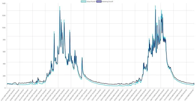
A series of experiments were conducted in the basins of Kosi region (Nepal) for 2 years in the period from 1997 to 1998. Experiment 1 was produced according to the catchment area of the Sagarmatha Post, the Dudh Kosi River and was conducted without changes in the initial param-eters in the software. For the target function, a multi-scale MSOF target function was adopted. The validation by the MSOF target function is 13.2, and the model call is 5829. The SLS calibra-tion was used. As can be seen in the graph (Fig.5), the flood recession is modeled well enough. This is relevant since it is the most accurate reflection of the different phases of the hydrological regime that is most important.
Experiment 2 was produced according to the catchment area of Kosi region (Nepal), the Sagar-matha Post, the Dudh Kosi River and was con-ducted without changes in the initial parameters in the software. Criteria and validation criteria
S/σ and S/σΔ were used for the objective func-tion and equal to 0.70. Calibrafunc-tion was performed using the Nelder-Mid method. As can be seen in the graph (Fig. 6), the flood recession is modeled somewhat worse for the selected period.
Importantly, the use of the MSOF functions in the calibration (for example, instead of the stan-dard deviation, criteria S/σΔ and S/σΔ and, as well as the Nash-Sutcliffe criterion), allows the user to pay attention to a very important effect: the simulated hydrograph approximates the actu-al vactu-alue as much as using these standard quadratic metrics [Sokolova and Kuzmin 2017].
CONCLUSION
“getting stuck” in the search for the optimum in insignificant “depressions”.
A method has been developed for presenting the results of the background forecasting of rain floods due to the fact that the applicant developed new MLCM3 software, based on the develop-ments of the RSHU and improved in the project “Development of methodological bases and man-agement technologies Water resources of river systems insufficiently illuminated by hydrome-teorological observations (on the example of the Mekong river basin)».
Acknoledgements
The presented work was funded by the Minis-try of Education and Science of the Russian Fed-eration (Project ID No. RFMEFI58316X0059;
the code of the application "2016-14-585-0005-002) within the framework of the Federal Target Program.
REFERENCES
1. Alfonso L., Jonoski A, Solomatin D. 2010. Multi-objective optimisation of operational responses for contaminant flushing in water distribution net
-works, Journal of Water Resources Planning and Management, 136(1), 48–58.
2. Barrett, D. 2008. Improved stream flow forecasting by coupling satellite observations, in situ data and catchment models using data assimilation meth
-ods, eWaterCRC Technical Report.
3. Burnash, R.J.C., R.L. Ferral, and R.A. McGuire, 1973. A generalized streamflow simulation sys
-tem – Conceptual modeling for digital computers.
Figure 5. Dudh Kosi, Kosi region (Nepal), from 01/01/1987 to 31/12/1988; Numerical experiments: SLS calibration, MSOF objective function
Technical Report, Joint Federal and State River Forecast Center, U.S. National Weather Service and California Department of Water Resources, Sacramento.
4. Johansson B. 1997, Development and test of the distributed HBV-96 hydrological model; Journal of Hydrology, 201 (1–4), 272–288
5. Kayastha N., Ye J., Solomatine D.P., Fenicia F., Kuzmin V. 2013. Fuzzy committees of specialized rainfall-runoff models: further enhancements and tests; Hydrology and Earth System Sciences, 11, 4441–4451.
6. Kuzmin V.A. 2001. Selection and parametrization of prediction models of river flow; Russian Meteo
-rology and Hyd-rology, 3, 64–68.
7. Kuzmin V.A. 2001. Short-term forecasting of di
-sastrous high waters and floods; Russian Meteorol
-ogy and Hydrol-ogy, 6, 67–71.
8. Kuzmin V., Seo D.-J., Koren V. 2008. Fast and effi
-cient optimization of hydrologic model parameters using a priori estimates and stepwise line search. Journal of Hydrology, 353(1–2), 109–128.
9. Kuzmin V.A. 2009. Basic principles of automatic calibration of multi-parameter models used in op
-erational systems of flash flood forecasting. Rus
-sian Meteorology and Hydrology, 34 (6), 384–391. 10. Pivovarova I.I. 2016. Optimization methods for
hydroecological monitoring systems. Journal of Ecological Engineering, 17(4), 30–34.
11. Phong V.V. Le, Kumar P, Dang H.V., Valocchi A.J. 2015. GPU-based high- performance computing for integrated surface-subsurface flow modeling. Environmental Modeling & Software, 73, 1–13. 12. Reed S., Koren V., Smith M., Zhang Z.. Moreda
F. 2004. Overall distributed model intercomparison project results, J. Hydrol., 298(1–4), 27–60. 13. Refsgaard, J.C. 1997. Parameterization, calibra
-tion, and validation of distributed hydrological models. Journal of Hydrology, 198, 69–97. 14. Sokolova D.V., Kuzmin V.A. 2017. Use of «MLCM3»
software for flash flood forecasting.,Conference pa
-per: European Geosciences Union General Assem
-bly 2017, Vienna, Austria http://meetingorganizer. copernicus.org/EGU2017/EGU2017–9498.pdf Ac
-cessed: 28 April, 2017.
15. World Meteorological Organization. Guide to Hy