Estimation of Plasma Emission Transition Using Hidden
Markov Model
∗
)
Shota NAKAGAWA
1), Teruhisa HOCHIN
1,2), Hiroki NOMIYA
1)and Hideya NAKANISHI
2)1)Kyoto Institute of Technology, Kyoto 606-8585, Japan
2)National Institute for Fusion Science, Toki 509-5292, Japan
(Received 27 December 2017/Accepted 8 August 2018)
This study proposes a method for estimating plasma-emission transitions from plasma-emission videos using a hidden Markov model (HMM). The proposed method retrieves similar videos and learns model parameters from them. The plasma-emission characteristics that we have employed are color, brightness, position, shape, and the speed at which the brightness of a plasma emissions changes. Multiple HMMs based on these plasma-emission characteristics are employed to represent the plasma-emission patterns. The anticipated plasma-emission transi-tions are estimated using state-transition probabilities from the generated model. Experimental results are used to confirm that the proposed methods are effective in identifying similar plasma videos and estimating probable future states of the plasma.
c
2018 The Japan Society of Plasma Science and Nuclear Fusion Research
Keywords: hidden Markov model, video, plasma, similarity, estimation DOI: 10.1585/pfr.13.3405117
1. Introduction
High-temperature plasma experiments are being con-ducted at the National Institute for Fusion Science (NIFS) [1]. During these experiments, emission is observed when the plasma reaches a sufficiently high temperature. The plasma emissions are recorded as videos and stored in disk storage at NIFS [2].
The future emission states of plasmas must be esti-mated to adjust experimental parameters for maintaining the plasma and making emergency stops to avoid the de-struction of devices. The durations of the plasma videos range from a few seconds to one hour and more than 100,000 stored videos are available. Predicting emission patterns from past data is difficult because it takes time to manually analyze numerous videos; therefore, a system must be developed to retrieve videos from past experiments that exhibit similar characteristics and use them to deter-mine the probabilities of future emissions.
The hidden Markov model (HMM) [3] is widely used to analyze time-series data [4, 5], particularly in the field of speech recognition, and is currently being used in other fields as well.
A method to use plasma videos to determine the prob-ability of future plasma emissions is proposed herein, and the effectiveness of the proposed method is confirmed. The feature values of plasma videos are defined; then, an HMM is used to classify the plasma videos based on their simi-larities. Plasma-emission models are then generated from similar videos to determine the emission patterns. Finally,
author’s e-mail: [email protected]
∗)This article is based on the presentation at the 26th International Toki Conference (ITC26).
the effectiveness of the proposed method is verified via an experiment.
The remainder of this paper is organized as follows. Section 2 provides an overview of this research. Section 3 describes the related study, and Section 4 proposes our method. Section 5 describes the experiment, Section 6 dis-cusses the results, and Section 7 concludes the study.
2. Overview of the Estimation Model
2.1
Plasma-emission videos
Plasma emission frequently occurs during high-temperature plasma experiments conducted at NIFS [1]. Video recordings of the plasma emissions are stored on disk storage at NIFS in the MPEG-1 format, with a frame rate of 29.97 frames/s. The width and height of a frame are 352×240 pixels. The durations of the videos vary, but most comprise approximately two hundred frames (∼7 s).
2.2
Overview of the plasma-emission model
The procedures used to construct our plasma-emission model are as follows. First, 148 videos are prepared. Sec-ond, the videos are divided intosegments that comprise multiple frames. For eachsegment, feature values are cal-culated. The videos are then categorized into 23 groups using HMM trained on the test videos. Then, the HMM pa-rameters are determined from thesegmentsin each group. Multiple HMMs are prepared by this procedure. Finally, for a prediction target video, the fitness to multiple HMMs is calculated. Then, the model representing the target video is selected.
c
2018 The Japan Society of Plasma
3. Related Study
3.1
Visual criteria for plasma videos
Evaluation criteria to determine the similarities among plasma videos have been proposed in reference [6, 7]: Cri. 1: Position of a bright spot
Cri. 2: Amount of movement of a bright spot Cri. 3: Expansion and contraction of a bright spot Cri. 4: Speed of brightness transition
Cri. 5: Amount of brightness transition Cri. 6: Color
Cri. 7: Amount of color transition
Some researchers in fusion science consider these fea-tures to be physically significant characteristics of plasma-emission phenomena [6, 7].
3.2
Frame-hashing method
A fast-detection method for querying streaming videos was proposed in reference [8]. The original frame-hashing method divides a frame into 4×4 blocks. The luminosity of each block is averaged and binarized using the mean luminosity of the frame. Thus, binary digits can be obtained for each frame, and this constitutes the “hash value” of a frame. The hash value can then be used to de-tect matching scenes in streaming videos.
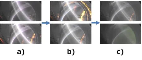
In this study, the frame-hashing method is used to di-vide a di-video intosegments. A frame is divided into 16×16 blocks for more accurate division. Asegmentis defined as a series of frames exhibiting similar hash values. Figure 1 shows sample frames in both same and differentsegments. Each column of frames corresponds to a differentsegment. The upper row is the first frame of asegment. In Fig. 1, the next frame after the lower frame of a) is the upper frame of b), and a similar pattern follows for columns b) and c). The lower frame of a) is noticeably different from the upper frame of b), even though these frames are adjacent to each other in the time series. It can thus be seen that frames are successfully divides frames intosegments, each of which contains similar frames.
3.3
HMM
An HMM is a generative probabilistic model, in which a sequence of observable variables is generated by a se-quence of internal hidden states. An HMM is based on
Fig. 1 Examples ofsegments.
two conditional-independence assumptions: 1) thetth hid-den variable,Qt, given the (t−1)th hidden variable, is in-dependent of the previous variables, and 2) thetth obser-vation,Ot, given thetthhidden variable, is independent of the other variables. These assumptions are qualitively rep-resented by Eqs. (1) and (2), respectively:
P(Qt|Qt−1,Ot−1, . . . ,Q1,O1)=P(Qt|Qt−1). (1)
P(Ot|QT,OT, . . . ,Qt, . . . ,Q1,O1)=P(Ot|Qt). (2)
Here,Qtis a discrete random variable withNpossible val-ues {1. . .N}, and T is the total number of observations. The hidden Markov chain defined byP(Qt|Qt−1), is
rep-resented by a stochastic transition matrix A = {ai,j} =
P(Qt = j|Qt−1 = i). The special case of time t = 1 is
described by the initial-state distributionπi = P(Q1 = i).
A particular sequence of observationsOis represented as O = (O1 = o1, ...,OT = oT). The probability that a
par-ticular observation vector occurs at a parpar-ticular timetfor a state jisbj(ot)=P(Ot=ot|Qt= j). The set of parameters is described asλ=(A,{bj(·)}, π).
Three basic problems are to be solved for an HMM: 1. FindP(O|λ) for someO=(o1, . . . ,oT).
2. Given someOandλ, find the best state sequenceq= (q1, . . . ,qT) that explainsO.
3. Findλthat maximizesP(O|λ).
A maximum-likelihood method of parameter-estimation to find the parameters of an HMM has been proposed in ref-erence [3]. In this study, we model the transitions between
segmentsusing an HMM.
4. Proposed Methods
4.1
Feature values
Four types of feature values are adopted: color, the amount of brightness transition (ABT), the speed of bright-ness transition (S BT), and theshape. These are defined by Eqs. (3) - (6), respectively.
Color(R,G,B)= 1
|F|
r∈F
|f(r)|. (3)
ABT=brightt−brightt−1. (4)
S BT =brightt−brightt−1
seg_num . (5)
S hape= 4π×area
circum f erence2. (6)
Here, f(r) is the pixel value at the coordinaterof the first frame of asegment. The quantityFis the sum of all pix-els in the first frame of asegment. We calculate the three
colors red, blue, and green. The quantity brightt is the
mean luminance value of the first frame of thetthsegment,
seg_numis the number of frames in the (t−1)thsegment,
Fig. 2 The model generated from a plasma video.
for eachsegment, six-dimensional features are used, and the feature values are calculated for eachsegment.
4.2
Plasma-emission model from an HMM
We model the transitions betweensegmentsin similar videos based on an HMM, and term the resulting model as the “plasma-emission model.” Figure 2 outlines a plasma emission model. The feature vector of asegment is re-garded as an observation vector ot, and a transition be-tweensegmentsis represented by a transition between hid-den states Qt. The observation vectors are continuous; therefore, the probability distributionP(ot|Qt) is assumed to be a mixture of multivariate Gaussians for each state.
4.3
Selection of similar videos
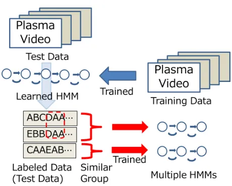
An HMM can determine the best state sequence q. The plasma videos can be converted into a symbol se-ries, which represents the series of hidden states q = (q1, . . . ,qT). Here, two or more plasma videos are
as-sumed to be similar when their symbol series are the same because the symbol series represent a time-series pattern. In this study, we used half of the prepared videos to train the HMM and employed the other half to test the trained HMM. For some videos, the videos are determined to be similar if three or more symbol series were the same; this number was determined experimentally. For example, as-suming that the symbol series for video S is (A,B,B,C,D) and that for video T is (E,A,B,B,C,A), videos S and T are similar because four symbol series (A,B,B,C) are the same. In this way, the prepared videos are categorized into several groups. We can then train the HMMs using sim-ilar videos and obtain multiple models that represent the plasma-emission pattern for each similar video. This pro-cedure is shown in Fig. 3.
4.4
Evaluation of the optimal model
An optimal plasma-emission model can be selected from the models obtained from a new video. Using the Viterbi algorithm [3], for each plasma-emission model, the tthstateqtfor thetthsegmentof a new video can be deter-mined.
We can calculate the Euclidean distance between the mean parameters µ = (μ1, . . . , μ6) for the tth state of a
plasma-emission model qt and the feature vector ot = (v1, . . . ,v6) for thetth segment of a new video. This
Eu-clidean distance is represented asdisj(t) (j=0, . . . ,22) for
Fig. 3 Generation of multiple models.
the plasma-emissionmodelj. When the values ofdisj(t) are arranged in ascending order, the ordered distance is de-noted byDisj,t(k), wherekis the order after sorting. For example, consider a case in whichmodel3 is the second
similar plasma-emission model to the 4thsegmentof a new video. In this case, dis3(4) is the Euclidean distance
be-tween the mean parameters of the fourth state of the third plasma-emission model and the feature vector of the fourth segment, andDis3,4(2) is the second distance among these
ordered values.
Let us consider the point at which the distance Disj,t(k+1)−Disj,t(k) becomes larger than the previous valueDisj,t(k)−Disj,t(k−1). We label this point asNt. The stateqtand the feature vectorotare regarded as simi-lar up toNt. The topNth
t plasma-emission models are then considered to be optimal for thetth segment of the new video.
For eachsegment, we calculate the value ofNt. For each plasma-emission model, thenumber of selections as
the top Ntthmodels(NST) is incremented according to the
segmentnumbert. The value of NST is considered to
rep-resent the similarity of the plasma-emission model to the new video. Figure 4 shows an example of the method for calculating NST. In this example because Models A and B are selected as the topNth
t plasma-emission models at time t, the NSTs of Models A and B are incremented. The same process is repeated for successive time increments. In this case, Model A is the most similar to the example plasma video because NST of Model A is the largest.
4.5
Determining the next emission
The transition probability can be obtained for each state; hence, the probable next state can be estimated from the current state. The symbol series are obtained from the plasma video used in the HMM; therefore, by obtaining the symbol series for the segment data used to train the plasma-emission model, it is possible to detect the types
Fig. 4 Method to calculate NST.
is composed of. The first frame of thissegmentis used as the representative frame for thesegment, and is used in the visualization of each state of the plasma-emission model.
5. Experiment
5.1
Experimental method
We prepared 148 videos, which we grouped into 23 plasma-emission models (model0-model22). We also
pre-pared three test videos (t1 to t3) to evaluate the proposed method.
We evaluated the plasma-emission model from two perspectives: 1) Has the appropriate plasma-emission model been selected for the test video from among mul-tiple models? 2) Does the plasma-emission model appro-priately predict future plasma emissions?
For each test video, we calculated the value of NST for each plasma emission model. Next, we compared the test video and the videos used in creating plasma models with an NST larger than unity. Next, we selected a plasma-emission model similar to the test video (Modelsim). This model was used to evaluate the response to perspective (1). Subsequently, we usedModelsimto predict a candidate for the probable next state to evaluate the response to perspec-tive(2).
5.2
Evaluation methods
We then examined whereModelsimis ranked in NST for eachsegment. We also evaluated the ratio of the num-ber ofsegmentsthat include correct candidate images pre-dicted in the top 80% of transition probability (Numcorrect) to the total number ofsegments(Numseg). The value ob-tained by dividingNumcorrectbyNumsegis called the “ratio of prediction” (RP), and is defined by Eq. (7).
RP= Numcorrect
Numseg . (7)
5.3
Results
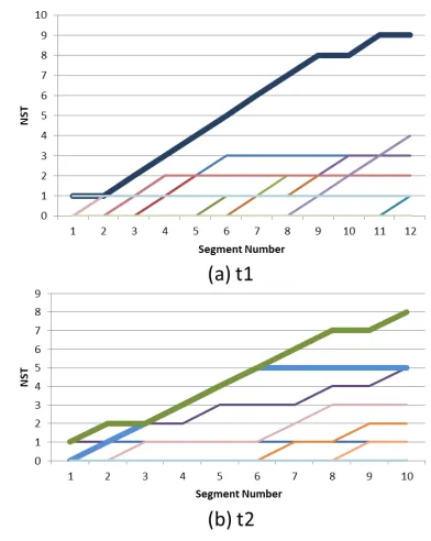
Figure 5 shows the values of NST for test videos t1 and t2 obtained through the method described above. The
Fig. 5 Transitions of NST persegment. Each colored line repre-sents a specific plasma-emission model. The bold lines are Modelsim, which adopts large values as compared
with the thin lines.
Table 1 Mean Rank ofModelsim.
Video Mean Rank Number ofsegments RP
t1 1.00 12 0.58
t2-1 1.00 10 0.20
t2-2 1.56 10 0.09
t3 2.10 11 0.09
vertical axis is NST, and the horizontal axis is the time in
asegment. The bold lines show Modelsim, and the thin
colored lines show other models. Each color represents a different model. The mean rank ofModelsimamong all 23 models is shown in Table 1, together with the correspond-ing value of RP.
As shown in Fig. 5,Modelsimis selected as an optimal model, rather than the other models; in the latersegments in particular,Modelsimhas a higher value of NST. For test video t2, two versions of Modelsim exist: t2-1 and t2-2. According to Table 1, the RP values are different for these test viedos. The mean rank ofModelsimis 1.42. This shows that the proposed method is effective in selecting the opti-mal model, even though the performance of the models is different.
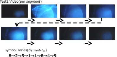
Examples of the first frames ofsegmentsand the se-quence of the symbol series for t1 and t2 are shown in Figs. 6 and 7, respectively. Examples of plasma-emission-model parameters are shown in Tables 2 and 4, respec-tively, while the mean parameters are shown in Tables 3 and 5, respectively. All mean values are normalized.
Fig. 6 Test video t1 and the corresponding symbol series.
Fig. 7 Test video t2 and the corresponding symbol series.
Table 2 Example of Plasma-Emission Transition (model17).
State
ID Features
Transition Probability
Transition Destination
0 Green, Bright 0.56 10
0.22 17
0.11 0
0.11 7
4 Red, Bright 0.50 4
0.50 15
10 Green, Bright 0.50 10
0.30 0
0.10 7
17 White, Bright 0.50 17
0.17 4
0.17 5
0.17 8
Table 3 Mean Parameters of Plasma-Emissionmodel17.
State
ID B G R ABT SBT Shape
0 1.10 1.68 1.03 0.23 0.40 0.74 4 1.10 0.65 1.61 -0.88 -1.01 0.50 10 0.93 1.58 0.87 -1.04 0.03 0.76 17 1.80 1.96 1.72 0.34 0.53 0.82
that the probability of transitioning from one bright emis-sion to another is high. For example, the probability of a transition from State ID 17 to 17 is high.
Figure 7 shows that even if the colors are the same,
manysegmentscan be decoded to different states. Table 4
shows that visually, many states have the same color.
Table 4 Example of Plasma-Emission Transition (model18).
State
ID Features
Transition Probability
Transition Destination
1 Blue, Bright 0.25 1
0.75 8
2 Blue, Bright 1.00 5
4 Blue, Dark 0.67 6
0.33 9
5 Blue, Bright 0.75 1
0.25 5
8 Blue, A Little Bright 0.25 2
0.75 4
Table 5 Mean Parameters of Plasma-Emissionmodel18.
State
ID B G R ABT SBT Shape
1 0.84 0.32 -0.84 -0.46 -0.06 1.06 2 1.37 0.58 -0.79 1.18 1.73 0.98 4 -0.57 -0.83 -1.09 -0.69 -0.75 1.11 5 1.49 0.85 -0.65 0.16 0.29 0.99 8 0.25 -0.31 -0.96 -0.51 -0.52 1.11
6. Discussion
According to Fig. 5, the differences among the values of NST are not large at the beginning of a video, but the value of NST for the bold line gradually increases more than those of the thin lines in the latersegmentsbecause a similar video has more similarsegmentsthan non-similar ones.
In test video t1, the plasma emissions are green, red, and white, and the duration of the bright emission is rel-atively longer than that for the other test videos. Hence,
thesegmentsfrom this video seem to be special. We can
actually observe the differences in the segmentsvisually. Conversely, in test video t2, the plasma emission is dark, and hence, visually selecting similarsegmentsis difficult. In Table 1, the mean RP is low. This indicates that many predicted images were different from the actual images. However, as RP is not 0 it can be seen that the image that is appropriately predicted was included in the prediction candidates.
We consider that the difference in the mean rank of each video and the value of RP are due to the pattern of the plasma emission.
7. Conclusion
In this study, we proposed a method for estimating plasma-emission transitions using an HMM trained on plasma-emission videos.
are well-classified. We conducted an evaluation experi-ment using the model rank results and showed that the op-timal model has a higher rank than others. We also con-ducted that acquiring knowledge about plasma emissions using the hidden Markov model is possible.
We plan future studies to improve this model and make it more robust to various emission patterns.
Acknowledgment
This research is partly supported by the National In-stitute for Fusion Science under NIFS15KLEH046.
[1] Large Helical Device Project Home Page, http://www. lhd.nifs.ac.jp/(reference 12-21-2017).
[2] M. Shoji, K. Yamazaki and S. Yamaguchi, “Development of the Real-time lmage Data Acquisition System for Observ-ing the Plasma Dynamic Behavior of LHD Long-pulse Dis-charges”, J. Plasma Fusion Res. SERIES3, 440 (2000). [3] J. Bilmes, “A gentle tutorial on the EM algorithm and its
ap-plication to parameter estimation for Gaussian mixture and
hidden markov models” (Technical Report ICSI-TR-97-02, University of Berkeley, 1997).
[4] H. Woo, Y. Ji, H. Kono and Y. Tamura, “Estimation Method for Lane Changes of Other Traffic Participants Using State-Unit based Hidden Markov Models”, Robotics Symposia proceedings21, 222 (2016).
[5] H. Ohya and S. Morishima, “Automatic Music Video Gener-ating System by Learning Existing Contents Based on Hid-den Markov Model”, Music and computer (MUS) Technical Report2012-MUS-95, 1 (2012).
[6] H. Shiroshita, T. Hochin, H. Nomiya and H. Nakanishi, “Similarity Retrieval of Plasma Videos and Its Evaluation”, Proc. of 3rd Int’l Conf. on Applied Comp. and Inf. Tech. (ACIT 2015), 229 (2015).
[7] H. Shiroshita, T. Hochin, H. Nomiya and H. Nakanishi, “Revised Similarity Retrieval Method of Plasma Emission Videos and Its Evaluation”, Proc. of 18th IEEE/ACIS Int’l Conf. on Softw. Eng., Artif. Intell., Networking and Paral-lel/Distr. Comp. (SNPD 2017), 575 (2017).