Array Antennas Based Joint Beamforming for IEEE 802.11n Wi-Fi

Array Antennas Based Joint Beamforming for IEEE

802.11n Wi-Fi

Cheng Guo, Liqiang Zhao

State Key Laboratory of Integrated Service Networks, Xidian University,

Xi’an, Shaanxi 710071, China [email protected]

Whai-En Chen

Dept. of Computer Science & Information Engineering National Ilan University

Taiwan [email protected]

Abstract—In order to achieve array gain and spatial diversity or

multiplexing gain simultaneously, a novel joint beamforming based on MIMO and array antenna techniques, referred to as J-BF, is proposed for the LTE and Wifi downlink. Array gain is achieved from array antenna based beamforming, referred to as AA-BF. Spatial diversity and multiplexing gains are achieved from MIMO based beamforming, referred to as MIMO-BF. To implement J-BF, i.e., joint AA-BF and MIMO-BF, an access point (AP) is equipped with separate array antennas. Before sending any data-frame in the J-BF mode, firstly, based on the estimated omni-directional CSI, the directional beam can be formed by the array antenna, and the array gain is achieved. Secondly, based on the estimated directional CSI, MIMO-BF is implemented to achieve the spatial diversity or multiplexing gain. More importantly, the J-BF algorithm maintains compatibility with 802.11n and there is not any change in terminals. Simulation results show that the proposed scheme can support the joint AA-BF and MIMO-AA-BF effectively and provide much higher array gain or spatial gains than the traditional MIMO or array antenna respectively.

Keywords: Beamforming; Array Antenna; MIMO

I. INTRODUCTION

Due to the demand for higher date rates in wireless communicaitons, some key technologies are proposed to enhance the capacity of wireless networks, e.g., LTE/LTE-A and Wi-Fi. MIMO precoding [1] is a very promising technology in LTE and Wifi, which is a multi-stream beamforming (BF) technique and can significantly improve system capacity and diversity gain, referred to as MIMO-BF [2]. MIMO-BF has demonstrated significant capacity improvement in scatter-rich wireless environments, e.g., the Rayleigh independent identically distributed (i.i.d) channel. In order to exploit the diversity or capacity gain in MIMO systems as large as possible, proper transmission precoding has been proved to be very effective under the condition that the channel knowledge information is available at the transmitter side[3]. Nevertheless, if the scattering is not rich enough at all, line-of-sight (LOS) component will be presented with a high probability, which can bring bad influence on MIMO-BF. As we all know, the LOS is a component that exists by virtue of a direct path between the transmitter and the receiver. And the LOS component manifests itself if the separation distance

between antennas is less than the coherent distance of the channel.

In the traditional array antenna based beamfroming, referred to as AA-BF [4], the same signal is emitted from each of the transmit antenna arrays with appropriate phase and amplitude so that the signal power is maximized at the receiver. AA-BF can enhance signal quality and increase system capacities without increasing the total transmit power [5]. Compared with MIMO-BF, AA-BF requires the LOS component, and the antenna arrays are closely co-located.

Hence, there is an urgent demand for joint beamforming, referred to as J-BF, to take full advantage of both AA-BF and MIMO-BF simultaneously in variable environments. In this paper, we present a J-BF strategy, i.e., joint MIMO-BF and AA-BF, for the LTE or Wifi downlink, which can provide spatial diversity, multiplexing gain and array gain simultaneously in different wireless environments. Moreover, the J-BF is implemented in the transmitter, i.e., access point (AP), and there is not any change in the receiver, i.e., mobile station (STA). The proposed J-BF is effective in both LTE/LTE-A and Wi-Fi, and for simplicity, we only consider implementing it in Wi-Fi in this paper.

The paper is organized as follows. The system model is introduced in Section II. The joint MIMO-BF and AA-BF algorithm is proposed in Section III. Simulation results are provided in Section IV. In Section V, the conclusion is given.

II. SYSTEM MODEL FOR JOINT BEAMFORMING

A. System Model

To take full advantage of both MIMO-BF and AA-BF simultaneously, each AP is equipped with NT array antennas,

each of which consists of Na arrays, as shown in Fig. 1. These

array antennas are well separated from each other by a distance Dc which exceeds the coherent distance of the channel. Moreover, in order to achieve the array gain as large as possible, the arrays within each antenna are highly close to each other [6]. According to the standard of Wifi, all STAs are equipped with NR omni-directional antennas.

QSHINE 2015, August 19-20, Taipei, Taiwan Copyright © 2015 ICST

Consider a signal vector s of dimensional NSS1 where

SS

N is the number of data streams. The signal vector is

multiplied by a matrix for MIMO-BF, _W_CNTNSS_{, and a} matrix for AA-BF, _V_CNTNaNT_{, prior to transmission. So} at the receiver, the received signal vector r of dimensional

1 

R

N is multiplied by the post-processing matrix P in order to extract the desired signal from the receiver perfectly, which can be expressed as:



HVWs n



P

Pr

s  

~ ₍₁₎

where the channel matrix _H_CNRNTNa_{, and the channel} noise _n_CNR1_{, which is drawn from an ensemble of i.i.d} complex Gaussian random variables with zero mean and variance_n2.

post-processing (P) MIMO-BF

(W)

AA-BF (V1₎

AA-BF (Vi₎

AA-BF (VNT₎ Nss data streams

NRomni-directional antennas

Na arrays of each antenna

NTarray antennas

S

STA

Fig. 1 System model for joint beamforming

The AA-BF matrix V could be expressed as:



T



a a

a

N N N

N

diag 1 _1, 2 _1,..., _1

 v v v

V , where i_N

a1

v is the AA-BF

vector of the i-th antenna at the transmitter. In order to constrain the total transmit energy, the matrix

satisfies

 

1 11 i N H i

N_a v _a

v , where

 

H denotes the conjugate transpose operator.

The channel matrix H is expressed as:

] ,...,

,

[ 1 2 T

a R a

R a R

N N N N N N

N   

 H H H

H , where i_{N N}

a R

H is the

channel matrix from the i-th antenna with Na arrays at the

transmitter to the receiver. For simple analysis, a set of channel models in Wifi [7], is given in Tab. 1.

TAB. 1 CHANNEL MODELS

RMS delay

Environment Example Model Spread (ns)

A 0 N/A N/A

B 15 Residential Intra-room, room to room C 30 Residential/small office Conference room, classroom

D 50 Typical office large conference room E 100 Large office Multi-story office F 150 Large space city square

III. JOINT BEAMFORMING ALGORITHM

At the beginning, the transmitter works in the omni-directional mode as it does not know both the MIMO-BF and

AA-BF matrix (i.e., W and V) corresponding to its receivers. Before calculating the two vital matrixes in the J-BF mode, the transmitter has to get the relevant CSI by which the W and V

can be naturally obtained. The reciprocity between the uplink and downlink channels can be exploited to achieve the CSI [8]. Please note that the required CSI for MIMO-BF and AA-BF is tremendous different.

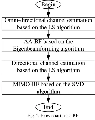
Omni-direcitonal channel estimation based on the LS algorithm

AA-BF based on the Eigenbeamforming algorithm

Direcitonal channel estimation based on the LS algorithm

MIMO-BF based on the SVD algorithm

Begin

End

Fig. 2 Flow chart for J-BF

To implement J-BF in the LTE downlink, as shown in Fig. 2, firstly, the AP estimates the CSI of the omni-directional channel through the uplink, and calculates the AA-BF matrix V

based on the estimated omni-directional CSI. Since then, the AP transmits its packets in the AA-BF mode. Secondly, after implementing AA-BF, the AP estimates the CSI of the AA-BF channel through the uplink, and calculates the MIMO-BF matrix W based on the estimated directional CSI. Finally, the J-BF is implemented and the benefits including diversity, array and multiplexing gains can be obtained through the J-BF mode eventually. The detailed steps are shown in the following:

 Omni-directional channel estimation

Wi-Fi is a typical OFDM-based packet transmission system, which divides the bandwidth into N orthogonal subcarriers. And the training symbols for N subcarriers can be obviously represented by the following diagonal matrix:

  

 

  

 

 

] 1 [ 0

0 ]

0 [

N X X

   



X (2)

where X[k] represents the training symbols at the k-th subcarrier, k0,1,2,...,N1 ,with E{X[k]}0 and

2

]} [

{X k x

Var  .

Given that the channel gain from the STA to the i-th antenna at the AP is Hi_{N N} [k]

R

              ] 1 [ ] 1 [ ] 0 [ N Y Y Y  Y =          

1] [ 0 0 ] 0 [ N X X                        ] 1 [ ] 1 [ ] 0 [ N H H H i N N i N N i N N R a R a R a  +            

1] [ ] 1 [ ] 0 [ N Z Z Z 

=XHi_{N N} Z

R

a (3)

where the channel vector i_{N N} R a

H from the STA to the i-th antenna at the AP can be expressed as:

T i N N i N N i N N i N

N_a _R[H _a _R[0],H _a _R[1],...,H _a _R[N1]]

H and the

noise vector Z[Z[0],Z[1],...,Z[N1]]T with E{Z[k]}0

and Var{Z[k]}z2.

In the following discussion, we assume that Hˆ denotes the

estimate values of the channel matrix i_{N N} R a

H . And the least-square (LS) estimation algorithm is used to get Hˆ in such a

way that the following cost function is minimized:

2

| |

| | 



  Y XH H）

（

J

=（YXH）H（YXH） (4) YHYYHXHHH XHYHH XHXH

By setting the derivative of the function with respect to Hˆ to zero, we can obtain

 

₂

_{ }

₂

_

_ˆ

_

₀

ˆ ˆ *       H X X Y X H

H H H

J

(5)

Hence,XHXHˆ XHY, which gives the solution to the LS estimation as

 

X X X Y X Y

H  H 1 H  1 (6) With respect to the reciprocity between the uplink and downlink channels, the downlink CSI from the i-th antenna at the AP to STA, i_{N N}

a R

H , can be represented as:

i_{N N} T

a

R （ ）



  H

H . (7)

 Array antenna based beamforming

There have been several effective AA-BF algorithms, e.g., direction-of-arrival (DOA) based beamforming [9] and eigenbeamforming[10], for the AP to get the directional beams

based on the estimated omni-directional CSI.

Eigenbeamforming takes full advantage of the spatial

correlations by transmitting over the strongest beam to a given user which can increase system capacity and reduce the interference from others, and we take it as the AA-BF algorithm in this paper.

Based on the estimated omni-directional CSI, the spatial correlation matrix between the i-th antenna of the AP and its STA is obtained as follows:





_

 

 _ i _

N N H i N N i a R a R

E H H

C i1,2,...,N_T (8)

The sorted eigenvalue decomposition of the correlation matrix Ci in the descending order is expressed as:

H i k N k i k i k H i i i i a ) ( ) ( _, 1 , ,D D

D Λ D C



 

  i1,2,...,N_T (9)

where D1,i corresponding to the largest eigenvalue λ1,i, is the

principal eigenvector of Ci.

In eigenbeamforming, the AA-BF vector of the i-th transmitter antenna at the AP, vi D_1,i.

 Directional channel estimation

Obviously, after implementing AA-BF, the channel has been changed seriously, which is not the initial omni-directional channel. So we have to estimate the CSI of the directional channel, referred to as HAA-BF, again. Similarly, it is

easy to estimate the AA-BF channel based on the LS algorithm as shown in the first step.

 MIMO based beamforming

Several effective MIMO-BF algorithms have being studied, e.g., Singular Value Decomposition (SVD) [11], Geometric Mean Decomposition (GMD) [12], etc. In this paper, we just take SVD into consideration.

The SVD of HAA-BF can be expressed as:



BF AA

-H UΣWH ₍₁₀₎

where U and W are unitary matrices; Σ is a diagonal matrix of the singular values of HAA-BF in the descending order. The

MIMO-BF matrix W _{is achieved now.}

Up to now, the AP has got the AA-BF and MIMO-BF matrix, and then sends its packets in the J-BF mode.

 Decoding

In order to decode the desired signal from each antenna at the STA, the received signal r should be multiplied by a weight matrix P such that

Pr s

~ ₍₁₁₎

Some popular decoding methods can be exploited to calculateP, e.g., the zero-forcing (ZF) and minimum mean square error (MMSE) algorithm recommended. In order to maintain compatible with 802.11n without any change in STA, the ZF is taken into account.







H







H

HVW HVW

HVW

P 1 (12) where()Hdenotes the Hermitian transpose operation. That is to say, it inverts the effect of channel as

n s Pr

s ~

~_{   (13)}

where ~nPn





HVW



HHVW



1



HVW



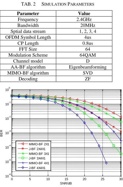
Hn. IV. SIMULATION RESULTS

In order to evaluate the proposed joint beamforming algorithm, the following simulations are performed under the indoor channel model D [13]. The values of the parameters used to obtain numerical results for simulations are specified in Wi-Fi, and some of the main parameters are given in Tab. 2. The distance between antennas at the AP is 0.5λ and that between arrays in an antenna is 0.25λ. For comparison, both the N_TN_aN_R J-BF system and N_TN_R MIMO system are evaluated under the same scenarios. For simplicity, we assume that both the AP and STA have the perfect CSI.

TAB. 2 SIMULATION PARAMETERS

Parameter Value

Frequency 2.4GHz

Bandwidth 20MHz

Sptial data stream 1, 2, 3, 4 OFDM Symbol Length 4us

CP Length 0.8us

FFT Size 64

Modulation Scheme 64QAM

Channel model D

AA-BF algorithm Eigenbeamforming MIMO-BF algorithm SVD

Decoding ZF

0 5 10 15 20 25 30 10-6

10-5 10-4 10-3 10-2 10-1 100

SNR/dB

BER

MIMO-BF 2X1 J-BF 2X4X1 MIMO-BF 3X1 J-BF 3X4X1 MIMO-BF 4X1 J-BF 4X4X1

Fig. 3 BER performance of J-BF with variable NT

The performance of J-BF using variable number of antennas at the AP is examined in Fig. 3, where the number of independent data streams is fixed at one. Obviously, the BER performance of J-BF increases with the increasing transmit antennas as it provides a larger diversity order of NT.

Unfortunately, due to only one antenna at the receiver, we cannot get any spatial multiplex gain under this scenario. On

the other hand, the performance of the N_TN_aN_R J-BF is

much better than that of the N_TN_R MIMO-BF as J-BF can obtain array gain to improve the link quality.

0 5 10 15 20 25 30 10-3

10-2 10-1 100

SNR/dB

BER

MIMO-BF 4X4 J-BF 4X2X4 J-BF 4X4X4

Fig. 4 BER performance of J-BF with variable Na

Fig. 4 shows that the performance of 4x2x4 and 4x4x4 J-BF is much better than that of 4x4 MIMO-BF as J-BF can achieve array gains by means of AA-BF. Moreover, the 4x2x4 J-BF scheme is 2 dB inferior to the 4x4x4 J-BF scheme as the latter one can obtain a greater array gain with a larger number of arrays. Compared with Fig.3, the number of independent data streams is 4 as NR=4 in Fig.4.

0 5 10 15 20 25 30 80

100 120 140 160 180 200 220 240 260

SNR/dB

Th

ro

u

g

h

tp

u

t(

M

b

it

/s

)

J-BF 2X4X2 MIMO-BF 2x2 J-BF 3X4X3 MIMO-BF 3x3 J-BF 4X4X4 MIMO-BF 4x4

Fig. 5 Throughput of J-BF with variable NR

Fig. 5 shows that system throughput of the 4x4x4 J-BF scheme is much higher than that of the 3x4x3 or 2x4x2 J-BF scheme as it achieves a greater spatial multiplex gain and can support up to 4 independent spatial data streams while the latter two schemes only support 2 and 3 spatial data streams, respectively. Moreover, system throughput of the 4x4x4 J-BF scheme is higher than that of the 4x4 MIMO-BF as J-BF can achieve array gains.

V. CONCLUSIONS

the omni-directional channel in the uplink, and calculates the AA-BF matrix based on the estimated omni-directional CSI. Since then, the AP transmits its packets in the AA-BF mode. Secondly, after implementing AA-BF, the AP estimates the CSI of the AA-BF channel in the uplink, and calculates the MIMO-BF matrix based on the estimated directional CSI. Hence, the J-BF algorithm is implemented, which is compatible with 802.11n. Simulation results show that after taking full advantage of both array antennas and MIMO, J-BF can provide a much lower BER than the conventional AA-BF and MIMO-BF respectively.

Currently, we are carrying out the following two researches. Firstly, we are researching adaptive beam- forming algorithms based on joint AA-BF and MIMO-BF. Secondly, in order to introduce the joint beamforming, we are researching enhanced SDMA protocols for 802.11n.

ACKNOWLEDGMENT

This work was supported in part by National Natural Science Foundation of China (No. 61372070), Natural Science Basic Research Plan in Shaanxi Province of China (2015JM6324), Hong Kong, Macao and Taiwan Science & Technology Cooperation Program of China (2014DFT10320), EU FP7 Project MONICA (PIRSES-GA-2011-295222), and the 111 Project (B08038).

REFERENCES

[1] H. K. Jayesh, K. B. Huang, MIMO precoding enable spatial multiplexing,power allocation and adaptive modulation and coding[p],US 7,702,029 B2,Apr. 20,2010.

[2] Y. P. Wu, C. K. Wen, C. S. Xiao, X. Q. Gao, R. Schober, Linear MIMO precoding in jointly-correlated fading multiple access channels with finite alphabet signaling, IEEE International Conference on Communications(ICC), pp. 5306-5311, 2014.

[3] D. R. Qin, Z. Ding, S. Dasgupta, On Forward Channel Estimation for MIMO Precoding in Cooperative Relay Wireless Transmission Systems, IEEE transaction on Signal Processing, pp. 1265-1278, 2014. [4] X. R. Wang, E. Aboutanios, M. Trinkle, M. G. Amin, Reconfigurable

Adaptive Array Beamforming by Antenna Selection, IEEE Transactions on Singal Processing, pp. 2385-2396, 2014.

[5] J. Singh, S. Ramakrishna, On the feasibility of beamforming in millimeter wave communication systems with multiple antennaarrays, IEEE transactions on Wireless Communications, pp. 1, 2015.

[6] R. A. Soni, R.M. Buehrer and R. D. Benning,”Intelligent antenna system for cdma2000,”in IEEE Signal Processing Magazine, vol.19,no. 4,pp. 54-67,2002.

[7] A. Stephens, B. Bjerke, etal.(2004).Usage Models,IEEE 802.11-03/802r23.

[8] T. Luo, A. Damnjanovic, Malladi, channel estimation for wireless communication[p], US 2011/006653 A1, Feb. 3, 2001.

[9] D. J. Yeom, S. H. Park, etal. Performance analysis of beamspace MUSIC withbeamforming angle, International Conference on Singal Processing and Communication Systems(ICSPCS), pp. 1-5, 2014. [10] J. Choi, On Coding and Beamforming for Large Antenna Arrays in

mm-Wave Systems, IEEE Wireless Communications Letters, pp. 193-196, 2014.

[11] H. Busche, A. Vanaev and H. Rohling, “SVD-based MIMO precoding and equalization schemes for realistic channel knowledge: Design criteria and performance evaluation,” in Wireless Personal Communications,vol. 48,no. 3,pp. 347-359,2009.

[12] Y. Jiang, J. Li and W.W. Hager,“Joint transceiver design for MIMO communications using geometric mean decomposition,” IEEE Trans. Signal Processing,vol. 53,no. 10,pp. 3791-3803,2005.