Re-identification of Vehicular Location-Based Metadata

(1)

Re-identification of Vehicular Location-Based

Metadata

Zheng Tan

1,∗

, Cheng Wang

1

, Weili Han

2

, Xiaoling Fu

1

, Jipeng Cui

1

, Changjun Jiang

1

1_{Tongji University, Shanghai 201804, China}

2_{Software School, Fudan University, Shanghai 201203, China}

Abstract

Amid the flourish of various data services, the privacy problems on metadata have received sufficient attention. Generally, the identity is the most sensitive attribute in metadata as identity is the key linking all attributes together. Thus, quite a few methods, such as dummy and k-anonymity, have been applied to actual applications to protect the identity . However, we still argue that the identity is very likely to be disclosed. In this paper, we study the re-identification problem in the seeminglyprivacy-preserving VLBS (Vehicular Location-Based Service). We find that the trajectories of vehicles are highly unique after studying 131 millions mobility traces of taxis. More specifically, the experiments demonstrate that only four spatio-temporal points are sufficient to uniquely re-identify the vehicle, achieving an accuracy of 95.35%. This indicates that there exists a high risk of re-identification in VLBS even identity has been protected by traditional methods.

Keywords: Privacy, VLBS, Re-identification, Uniqueness, Trajectories

Copyright © 2017 Zheng Tan et al., licensed to EAI. This is an open access article distributed under the terms of theCreativeCommonsAttributionlicense(http://creativecommons.org/licenses/by/3.0/),whichpermitsunlimited use,distributionandreproductioninanymediumsolongastheoriginalworkisproperlycited.

doi:10.4108/XX.X.X.XX

1. Introduction

Benefiting from yielding implicit information about individuals, large-scale data sets of human behavior play an important role in various network services, such as Location-Based Services (LBS)[1,2], Recommending System and Authentication System. Accompanied with the convenience, privacy concerns also deserve attention as the captured data always contain large amounts of personal private attributes, including location, identity, age, etc. Note that the identity is the most sensitive information among various personal attributes because of two reasons: (1) Based on the identity, other attributes can associate with each other objectively. The identity disclosure always gives rise to leaking a series of personal attributes. (2) To trace to its source, privacy is an subjective concept. The identity is the most intuitive sensitive information for ordinary people. Thus, in this paper we aim at revealing the identity disclosure, namely, the re-identification problem. Moreover, we carry out our work in the

H_{This paper’s earlier version was presented at 2016 International}

Conference on Security and Privacy in Communication Networks, Guangzhou, Oct. 10-12, 2016.

∗

Corresponding author. Email:[email protected]

background of LBS[3–6], which is widely used but tortured by re-identification problem.

In an LBS system, LBS providers/servers are often regarded as non-trustworthy components that perhaps leak users’ information to the third party deliberately or unintentionally. To improve their reliability, the servers usually anonymize the data to protect users’ privacy, [7–

9]. Under such anonymous protection, if an adversary hacks into an LBS server to get its trajectory metadata, he/she usually can only obtain an anonymous trajectory dataset, and cannot infer an individual’s trace from the anonymous data. As a result, a completely anonymous dataset is often presumed to beslightly sensitive when only several non-anonymous records of a specific user could be exposed to adversaries, [10]. The objective of our work is to probe the possibly “hidden” privacy leakage problem of user’s re-identification in LBS.

More specifically, we intently investigate the user’s re-identification problem for a special type of LBS, Vehicular Location-Based Service (VLBS). The reasons why we focus on VLBS are two-fold: Firstly, VLBS is becoming a promising type of location-based services, since more and more vehicles are able to access the Internet as mobile terminals, and then many LBS-related applications are devised to serve vehicles. For example, a transportation monitor application

EAI Endorsed Transactions

on

Security and Safety

Research Article

(2)

Zheng Tan, Cheng Wang, Weili Han, et al.

[11] collects real-time vehicle location information to predict road condition and generate suggestions to drivers. Secondly, a significant feature of VLBS, i.e., the mobility traces of vehicles are usually constrained by roads, draws us to figure out whether road information could improve the risk of user’s re-identification. To the best of our knowledge, few researches distinguished the privacy issue of VLBS as an independent problem from the LBS privacy problem, [12–14].

In this paper, we utilize non-sensitive datasets to evaluate whether they can still cause privacy leakage problems (user’s re-identification) in VLBS. To be specific, we extract a few non-anonymous trajectories from two datasets of taxi trajectory metadata, 131 millions mobility traces of taxis in Shenzhen and 1.1 billions of taxis in Shanghai, and compute the uniqueness of taxi trajectories. Surprisingly, we find that four spatio-temporal points are sufficient to identify vehicles even when anonymous protection strategies are adopted, achieving an accuracy of 95.35% for Shenzhen dataset and 96.75% for Shanghai dataset respectively. Experiment results show that vehicles trajectory privacy is inclined to be risky. We provide an intuitive explanation for this observation as follows: Compared with diverse human trajectories, vehicle traces are mostly binded by roads. The road information is possibly the underlying reason for user’s re-identification only by four record points.

The rest of this paper is organized as follows: Section

2 introduces related work in LBSs and VLBSs privacy fields. Section3gives the main results of this work. In Section4, we provide the analyzing procedure based on two real-life datasets. Section5 makes a discussion on what insights can be obtained from the experimental results. Section 6 draws a conclusion and discusses about the future work.

2. Related Work

One of the classic privacy protection mechanisms is the

k-anonymous algorithm [15–21]. In the model, a dataset

must have k undistinguishable items on a specific property, where k infers the least risks that we can suffer when information is leaked. At the beginning, the algorithm was designed for databases like hospital and school for user privacy protection. Later, researchers found thatk-anonymity can also work effectively in the LBS privacy protection.

To disclose the risk of user’s re-identification in anonymous dataset, Montjoye et al.[22] studied the uniqueness of shopping mall metadata. The shopping mall metadata has four fields: anonymous ID, time, location and money spent by that customer. In their experiments, they applied different resolutions to all fields except ID to simulate basic privacy protection methods. The conclusion is that four purchase records

are enough to uniquely re-identify 90% individuals. This result is achieved with metadata that has three dimensions (purchase time, shop, price). If an individual is re-identified, his/her mobility traces corresponding to purchase behaviors can be inferred by adversaries. To explain this result, an underlying reason is that the relatively high dimension of metadata could expose individuals’ privacy with a high accuracy. Another similar work [23] studied the uniqueness of human traces associated with phone activities. They use anonymous mobile phone dataset for their experiments. When people use their phones (to make a call or send a message), the phone will communicate with the nearest antenna and the whole activity is recorded by telecommunication company. There are three fields in their dataset: anonymous ID, the beginning time and antenna used (location, one antenna covers a specific area). Similarly, they applied different resolutions to the time and location fields. The result shows that four phone activities are enough to uniquely identify 95% individuals. If an individual is re-identified using the dataset, his/her mobility traces corresponding to phone activities are exposed to adversaries. Compared to the shopping mall metadata which has three dimensions, this work just use a two-dimension metadata. We notice that the location information of user is indeed represented by the coverage area of corresponding antenna. In other words, adversaries are just aware of which antenna the individual has communicated with. An antenna covers a large area, so privacy problem in this two-dimension metadata seems not that critical.

In our problem, the taxi trajectory metadata has two dimensions: LBS query time and position. Such a low data dimension makes the privacy problem seem less serious.

3. Main Results

3.1. Four Points for Re-Identification

In LBS, application server stores records of users, including ID, time and location information. We cannot infer one’s real identity by ID, since ID is anonymously stored in the server. For example, when we use Google Maps [24] for navigation, Google just uses our Google account as ID, so the application will never know our identities or the plates of our cars. Although this basic mechanism protects our privacy to some extent, the LBS servers are still considered unreliable.

(3)

Re-identification of Vehicular Location-Based Metadata

Temporal Resolution (min)

20 30 ₆₀ 80 120 240 Spatial Resolution 200 90 100 8070 6050 4030 2010

Uniqueness of traces

0.0 0.2 0.4 0.6 0.8 1.0

4

(a)N=4

20 30 60 80 120 240 Spatial Resolution 200 90 100

80706050 40302010

0.0 0.2 0.4 0.6 0.8 1.0

1

(b)N=1

807060504030 2010

0.0 0.2 0.4 0.6 0.8 1.0

2

(c) N=2

20 30 60 80 120 240 Spatial Resolution 200 90 100 8070 605040302010

0.0 0.2 0.4 0.6 0.8 1.0

3

(d)N=3

80706050 4030

2010

0.0 0.2 0.4 0.6 0.8 1.0

5

(e)N=5

20 30 60 80 120 240 Spatial Resolution 200 90 100 8070 6050 4030 2010

0.0 0.2 0.4 0.6 0.8 1.0

6

(f)N=6

80706050 40302010

0.0 0.2 0.4 0.6 0.8 1.0

7

(g) N=7

Figure 1. The Result of Shanghai’s Taxis.

of the car at any moment. Generally, one spatio-temporal point is enough for re-identifying a target if its trajectory is without an anonymous protection. In our experiments, we attempt to figure out the risk of being re-identified with basic generalization protection methods. Generalization also helps to eliminate spatial and temporal error because the adversaries cannot record spatio-temporal points without any error. It is achieved by spatial and temporal resolution. The details will be explained in Section4later.

In our experiments, we have 6 levels (20, 30, 60, 80, 120, 240 minutes) of temporal resolutions and 11 levels (10×_{10, 20}×_{20, ..., 100}×_{100 and}

200×_{200 blocks) of spatial resolutions. Besides, 1}∼₇

spatio-temporal points are randomly sampled for our matching experiment respectively. The three mentioned parameters have 462 (6×₁₁×_{7) combinations in all.}

For each combination, we obtain 150,000 samples and for each sample we test its uniqueness. By this procedure, we can compute the proportion that a taxi can be uniquely identified. Figure 3 illustrates the uniqueness of traces when we set the temporal resolution to 20 minutes and spatial resolution to 100×

100 square blocks. We can observe that the uniqueness grows rapidly as the number of known spatio-temporal

20 30 ₆₀ 80 120 240 Spatial Resolution 200 90 100 8070 6050 4030 2010

0.0 0.2 0.4 0.6 0.8 1.0

4

(a)N=4

807060 5040302010

0.0 0.2 0.4 0.6 0.8 1.0

1

(b)N=1

80706050 40302010

0.0 0.2 0.4 0.6 0.8 1.0

2

(c) N=2

80706050 40302010

0.0 0.2 0.4 0.6 0.8 1.0

3

(d)N=3

80706050 40302010

0.0 0.2 0.4 0.6 0.8 1.0

5

(e)N=5

80706050 40302010

0.0 0.2 0.4 0.6 0.8 1.0

6

(f)N=6

80706050 40302010

0.0 0.2 0.4 0.6 0.8 1.0

7

(g)N=7

Figure 2. The Result of Shenzhen’s Taxis.

1 2 3 4 5 6 7

The number of spatio-temporal points 0.0 0.2 0.4 0.6 0.8 1.0

Shanghai Shenzhen

Figure 3. The Uniqueness of Traces with A Specific Number of

Known Non-anonymous Spatial-Temporal Points. Given a100×

100 spatial resolution and20 minutes temporal resolution, the

uniqueness is up to 95.35% for Shenzhen taxis and 96.75% for Shanghai’s, when the number comes to 4.

(4)

0

1

2

3

4

5

6

7 Number of spatio-temporal points

0.0

0.2

0.4

0.6

0.8

1.0 Uniqueness of traces

TR

20 30 60 80 120 240

0

1

2

3

4

5

6

7 Number of spatio-temporal points

0.0

0.2

0.4

0.6

0.8

1.0 Uniqueness of traces

TR

20 30 60 80 120 240

0

1

2

3

4

5

6

7 Number of spatio-temporal points

0.0

0.2

0.4

0.6

0.8

1.0 Uniqueness of traces

SR

200 100 90 80 70 60 50 40 30 20 10

0

1

2

3

4

5

6

7 Number of spatio-temporal points

0.0

0.2

0.4

0.6

0.8

1.0 Uniqueness of traces

SR

200 100 90 80 70 60 50 40 30 20 10

(

a

)

U

−

TR

−

NoST

of Shenzhen

(

b

)

U

−

TR

−

NoST

of Shanghai

(

c

)

U

−

SR

−

NoST

of Shenzhen

(

d

)

U

−

SR

−

NoST

of Shanghai

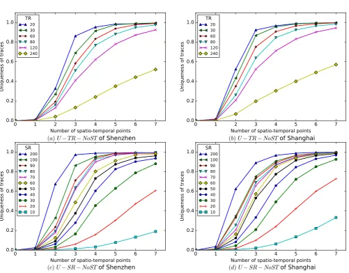
Figure 4. The Impacts of Temporal and Spatial Resolutions on The Uniqueness. Figure (a) and (b) show how different levels of temporal resolutions affect the uniqueness. Figure (c) and (d) show the effects of different spatial resolutions on the uniqueness. The

notations U, TR,SR, NoST stand for Uniqueness of traces, Temporal Resolution, Spatial Resolution, Number of Spatio-Temporal

points, respectively.

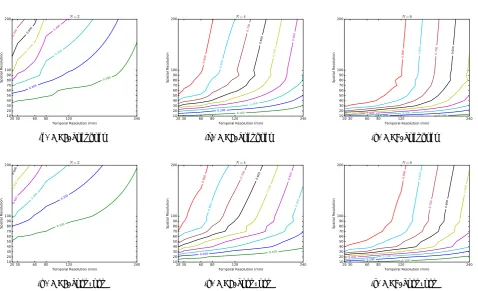
In order to find out the effects of the temporal and spatial resolution on the uniqueness of traces, we conduct experiments with different temporal and spatial resolutions. The results are shown in Figure 4. By these, we can conclude that the uniqueness benefits from a larger number of spatio-temporal points, a shorter temporal resolution, and a bigger spatial resolution (i.e., a smaller block size). Furthermore, in Figure 5, we plot the contour map according to the uniqueness of traces extracted from two cities with the given known points 2, 4 and 6.

For each given number of spatio-temporal points, we plot the uniqueness of two datasets in Figure 1

and Figure 2, corresponding to changing temporal and spatial resolutions. When the number of spatio-temporal points equals to 1 (N = 1, Figure 1(b),2(b)), the surface is nearly flat, which means that a single point is insufficient to re-identify a taxi, whatever the

temporal and spatial resolutions are given. With the growing ofN, the re-identified accuracy (uniqueness) is increasing rapidly. WhenN equals to 4 (N = 4, Figure

1(a), 1(a)), moderate temporal and spatial resolutions can lead to a uniqueness over 90%. And the uniqueness exceeds 90% for most temporal and spatial resolutions whileN equals to 7 (N = 7, Figure1(g),2(g)).

In both datasets, the trajectories cover square areas with a side length of 200 kilometers, spreading over two degrees in longitude and latitude. If the spatial resolution is chosen to be 10×_{10, then we get 100}

square blocks, with a 20-kilometer side length for each. Such a block is much too huge for estimation. The appropriate and practical resolution is 100×_{100, which}

(5)

20 30 60 80 120 240

Temporal Resolution (min) 10 20 30 40 50 60 70 80 90 100 200

Spatial Resolution 0.100

0.200 0.300 0.400 0.500 0.600 0.700

N= 2

(a)N=2, Shanghai

20 30 60 80 120 240

Temporal Resolution (min) 10 20 30 40 50 60 70 80 90 100 200 Spatial Resolution 0.100 0.200 0.300 0.400 0.500 0.600 0.700 0.800 0.900

N= 4

(b)N=4, Shanghai

20 30 60 80 120 240

N= 6

(c) N=6, Shanghai

20 30 60 80 120 240

Temporal Resolution (min) 10 20 30 40 50 60 70 80 90 100 200

Spatial Resolution 0.100

0.200

0.300

0.400 0.500

0.600

N= 2

(d)N=2, Shenzhen

20 30 60 80 120 240

N= 4

(e)N=4, Shenzhen

20 30 60 80 120 240

N= 6

(f)N=6, Shenzhen

Figure 5. Contour Map of Uniqueness of Traces of Two Cities.

3.2. Time Closeness

Based on the above conclusions, we further investigate on the temporal correlation between the four obser-vation points. As all users are restricted to the road network in VLBS, one vehicle’s moving trace is most likely to be analogous to his adjacent vehicles for some time, especially during the rush hours. Intuitively, if the observing time of the four points is too close, obtaining four points are not enough to distinguish one vehicle from others. To validate this supposition, we carry out the following experiments.

Firstly, we extract the feature to characterize the closeness degree of the four points To formulate, we assume that the time stamps of the four points is denoted by T ={_T₁_{, T}₂_{, T}₃_{, T}₄}_{. Without loss of}

generality, we regard that the four time stamps are in chronological order. Then we define the average time difference between two adjacent time stamps as the closeness degree, shown as

C =T4−T1

3 (1)

Specially, in the above setting, we choose n points randomly as the observing points. We can regard their time stamps as the dots sampled from a Uniform DistributionU(0, θ). Then the difference between two adjacent time stamps, D={_d_ij ₌_T_i−_T_j | _i−_j_{= 1}}_{, is}

subject to the following probability density function,

f(d) = n!

θn_(j−_i−_1)!(n−_j₊_i)!d

j−_i−₁

(θ−_d)n−j+i ₍₂₎

And the expectation ofDis shown as follow,

E(D) = θ(j−i)

n+ 1 (3)

Actually, the expectation can be regarded as the closeness degree of the random selection CR. In our experiments, the four points can re-identify one vehicle in one day’s traces randomly. Thus we can obtainCR= 4.8hasθ= 24handn= 4.

Next we carry out a series of experiments, illustrated by Fig.6and7. Taking Fig.6as an instance, we calculate the uniqueness withC={_0.5,_1,_2,_4.8,₆}_while_N _takes

4. Apparently, the uniqueness increases along the close-ness degree grows and reveals convergent tendency whenC≥_{2. Moreover, the figure of uniqueness in}_C₌

4.8 is similar to the that of the random selection( shown in fig. 1(a)). Our experiments validate that the time closeness of observation points can indeed influence the uniqueness.

4. Investigating Procedure

(6)

30min

1h

2h

4.8h

6h

Closeness degree

Figure 6. The Uniqueness of Traces with different closeness degree in Shanghai. Note that the observation points countN takes 4.

30min

1h

2h

4.8h

6h

Closeness degree

Figure 7. The Uniqueness of Traces with different closeness degree in ShenZhen. Note that the observation points countN takes 4.

steps: pre-processing, temporal generalization, spatial generalization and uniqueness calculation. During pre-processing, datasets are processed to satisfy the require-ments of experirequire-ments. Temporal generalization applies a specific resolution to the time field. For adversaries, points within a resolution cannot be distinguished. Similarly, spatial generalization applies a resolution to the location field. After temporal and spatial general-ization, the last step is to find out the possibilities that one taxi can be re-identified uniquely by adversaries given specific number of spatio-temporal points. When carrying out the experiment, we test different temporal and spatial resolutions with different number of spatio-temporal points.

The details of each step are shown in the following sections. We will give an overview of our datasets at the end.

4.1. Dataset Pre-processing

The two adopted datasets take about 60 Gigabytes disk storage in all. The data get a lot of redundances and mistakes when taxi companies record and store them.

Before implementing the experiments, we have to do some pre-precessing work to clean the datasets.

In the first step of pre-processing, redundant fields are removed. Besides redundant data, logs can also have minor mistakes. The data contains broken records, such as those with temporal disorder and spatial misplace.

Records in datasets are expected to be temporally well organized, but some of them are chronological disordered. When such a temporal disorder takes place, uncorrelated points may occur in the chronological sequences (as is shown in Figure 8(a)). All of the temporal uncorrelated points in the logs should be removed in this stage. Another temporal disorder case is that all the point sequences are correlated with each other, but some of them are shifted (as Figure

(7)

t

i

t

i

t

i

t

i

t

i

t

k

t

(a)

t

i

t

i

t

i

t

i

t

(b)

Figure 8. Illustration of Temporal Disorder. In Figure8(a), on the

road segment fromBtoE, there are several points amongti and

ti+5, andtk’s temporal tag doesn’t match the surrounding points’

tags, which makes it a broken point. So tk should be removed

in the pre-precessing stage. In Figure 8(b), t3 shifts ahead t2

(or t2 shifts behind t3). Two solutions are used for solving this

temporal error. One is removingt2 or t3, the other is correcting

t2’s ort3’s temporal tag. Both solutions need the average speed

parameter as a reference.

The last case is spatial displace. When taxis report their locations to the server, they upload their longitude and latitude information, and the server receives and stores this information into database. The whole process can not be done perfectly. The bits representing the longitude and latitude may be changed when the location information is being transmitted and stored, which leads to spatial displace. Spatial displace makes one point from the sequences shift away from others, as is shown in Figure 9. After calculating the speed between points, a point spatial displace can be distinguished if its speed to adjacent points is extremely large. Spatial displaced points will be removed from the records.

i

t

i

t

i

t

i

t

i

t

i

t

i

t

i i

v

i i

v

i i

v

Figure 9. Illustration of Spatial Misplace.ti+3 has a deflection

from the main road, which can be tested by communication error between GPS devices and GPS servers. The average speed is

calculated for finding the deflection points. In the figure,vi+2,i+3

is the average speed betweenti+2 andti+3, and so arevi+3,i+4

and vi+2,i+4. By comparison, vi+2,i+3 and vi+3,i+4 are much

more larger thanvi+2,i+4. Frequently their values exceeds taxis’

maximum speed. So we can considerti+3 as an invalid point and

remove it from logs.

In the end, some taxis have only a small number of records, so they are not suitable for the experiments. These cars are simply removed from logs.

4.2. Temporal Generalization

Take Shenzhen taxis data as an example, whose timeline covers 9 days. In temporal generalization step, different levels of temporal resolutions are tested in our experiments. A specific temporal resolutiontr will divide the whole timeline (9 days, 12,960 minutes) into 12,960/tr periods. In Figure 10, the spatio-temporal points are mapped to each interval according to their temporal tags. By doing so, points nearby are classified to the same period. Thus, the adversaries can not tell the temporal differences among the points within the same period.

Actually, two time-related concepts are involved in our attacker model, say, the Adversary spying time (AST) and the Server recording time (SRT). AST is the time that adversaries record when following a car, while SRT is the time that the server records when a car starts a query to server. In fact, the adversary can not obtain the query start time (QST) easily and the QST also has a numerical difference from the AST. These two reasons make a unstable numerical difference between AST and SRT. In our experiments, we set temporal resolutions to simulate the situations that AST has a shift from SRT.

(8)

7UDMHFWRU\ LQWZR

KRXUV

$YHUDJH*36 SRLQWDFFRUGLQJ WRWKHUHSRUWHG *36SRLQWVLQ KDOIRIDQKRXU

5HSRUWHG *36SRLQW

$

% &

5HSRUWHG *36SRLQW 7UDMHFWRU\LQ

WZRKRXUV

'

Figure 10. Illustration of Temporal Generalization. The gray line is the trajectory of a car in timeline from 10:00 to 12:00. In temporal generalization process, we set the temporal resolution to half an hour, and the path is divided into 4 periods marked by different colors. Points in the same period are

considered undistinguishable. For example,AandB,CandDare

undistinguishable, whileAand C,Band Dare distinguishable.

7UDMHFWRU\ LQWZR

KRXUV $YHUDJH*36

SRLQWDFFRUGLQJ WRWKHUHSRUWHG *36SRLQWVLQ KDOIRIDQKRXU $

%

& _'

Figure 11. Illustration of Spatial Generalization. The entire area

is divided into6×₆_{blocks bounded by yellow and gray dotted}

lines. After the spatial generalization, Aand B are in different

blocks, while C and D are in same block. So A and B are

distinguishable, C and D are undistinguishable. We say that

the6×₆_{spatial resolution cannot tell}_C _from_D_{. When spatial}

resolution level is reduced to 3×₃ _{(divided by yellow dotted}

line),B is mingled withC andD.

4.3. Spatial Generalization

The Shenzhen and Shanghai taxis’ trajectories both cover an approximate square area that spreads over 2◦ in longitude and 2◦ in latitude. In this stage, we use a simple and direct way to generalize the spatial area. We draw lines with different densities along the longitude and latitude lines and divide the entire mobility spatial area into different blocks.

As shown in the Figure 11, points in the same blocks are identical in their location when exposed to adversaries. This method of division can simulate k-anonymous algorithm to some extent, while pure k-anonymous division will create dynamic districts as time goes by. With the source dataset, we can not locate the precise position of all taxis at a specific time, which means that the pure k-anonymous algorithm is impractical. In our experiments, different division densities are set to replace different values of k’s in k-anonymous algorithm. The more blocks are divided, the smaller each block is. We apply 11 different spatial resolutions in the experiments (10×_{10, 20}×_20,...,

100×_{100, and 200}×_200).

4.4. Uniqueness Calculation

After pre-processing, temporal generalization and spatial generalization, we can calculate the uniqueness of a taxi’s trajectory. LetUs denote the uniqueness of a trace given several known spatio-temporal points. We also define uniqueness indicator, which indicates the possibility that a trace can be identified with a specific number of spatio-temporal points.

Us=

(

1 if a sample is unique, 0 otherwise.

In Figure 12, when the number of known spatio-temporal points is 2 (points B and C here), the value ofUsis 0 according to the above formula. If 3 points are known (eitherA,B,CorB,C,D), thenUsequals 1.

Now that we can calculate the value of Us given several spatio-temporal points, the last problem to solve is how to get enough samples of several spatio-temporal points. We use statistical approaches to sample from the taxis’ records repeatedly, and match it with the entire dataset to calculateUs. With enough samples, the uniqueness indicator can be inferred as in Equation (4).

=

P s∈_SUs

|_S| ×100% (4)

In our experiments, we mainly have 3 variables (the temporal resolution TR, the spatial resolutionSR, and the number of known spatio-temporal pointsN). Please refer to the detailed results of our experiment and the relations betweenand the three variables can be found in Section3.

Algorithm 1gives the procedures of computing the uniqueness of users’ traces.

4.5. Datasets Overview

(9)

7UDMHFWRU\ LQWZR

KRXUV

$ %

& '

( )

*

+

Figure 12. Illustration of Uniqueness Judgement. The blue and red lines are trajectories of two taxis with a timeline from 10:00

to 12:00, A and E turned out to be in period 10:00 to 10:30

(similarly, B and F in period from 10:30 to 11:00; C and G

in period from 11:00 to 11:30; D and H in period from 11:30

to 12:00). Given 2 spatio-temporal points,B and C, we cannot

identify the blue line trajectories. But if additional points, Aor

D or both of them, are given, this trajectory can be uniquely

identified.

Table 1. Overview of Datasets

Index Date #Taxis #Records

Shenzhen 2011

04/18˜04/26

13798 130,551,644

Shanghai 2015

04/01˜04/10

13899 1,141,606,183

identification of taxis. Time is the time when the taxi reports its location to LBS server.LongitudeandLatitude denote the location of a taxi.

In our datesets, each taxi has plenty of records every day, and more records mean that a taxi has more trajectory data. Figure13gives the probability density distribution of the number of taxi trajectory records per day. We can see from the figure that the probability density of Shanghai dataset is increasing with the growing number of records while that of Shenzhen dataset is decreasing. Taxis in Shanghai tend to have more trajectory records per day than those in Shenzhen.

Actually, a larger number of records do not mean more trajectory information. For example, given the same number of trajectory records, those with larger time-span may contain more information. Figure 14

gives the interval length distribution of two adjoined records. As we use taxi trajectory data from taxi companies instead of private cars, and taxi companies often collect their taxis’ location diligently, more than

Algorithm 1Computing Uniqueness of Traces

Require:

The entire original datasets,DSo.

Ensure:

A list with result tuples which contain parameters and the value of uniqueness,R.

1: Clean the original datasetDSowith methods in pre-preprocess stage, getDSc.

2: InitializeRwith an empty list. 3: InitializeCountwith 150,000.

4: foreachTR∈_[20,_30,_60,_80,_120,_240]_do

5: foreachSR∈_[10,_20,_30,_40,_50,_60,_70,_80,_90,_100,_200]

do

6: Divide theDScwithTR,SR, getDSd. 7: foreachN ∈_[1,_2,_3,_4,_5,_6,_7]_do

8: c= 0

9: m= 0

10: whilec <Countdo

11: SampleN spatio-temporal pointsPn from DSc

12: iflen(matched(Pn,DSd)) == 1then

13: m+= 1

14: end if

15: c+= 1

16: end while

17: =m/Count

18: R.append((TR,SR,N,))

19: end for

20: end for

21: end for

22: return R

Table 2. Data Sample from Shenzhen’s Taxicab

ID Time Longitude Latitude

B00T12 2011/04/18 00:00:18

113.98456622.560133

B00T12 2011/04/18 00:01:14

113.99459822.556467

... ... ... ...

B001B2 2011/04/20 00:01:55

113.88169922.742943

B001B2 2011/04/20 00:02:55

113.88086722.739964

... ... ... ...

B02S48 2011/04/23 19:54:42

114.26241322.711182

B02S48 2011/04/23 19:55:22

114.26193222.715206

B02S48 2011/04/23 19:56:39

114.26151322.718210

... ... ... ...

(10)

0 1000 2000 3000 4000 5000 6000 7000 8000 9000 Number of records

10-4

10-3

10-2

10-1

100

Probability density function

Shanghai Shenzhen

Figure 13. Probability Density Function of the Average Number of a Taxi Trajectory Records Per Day.

0 2 4 6 8 10 12 14 16 18 20 Interval length (h)

10-8

10-7

10-6

10-5

10-4

10-3

10-2

10-1

100

101

Probability density function

Shanghai Shenzhen

Figure 14. The Distribution of Interval Length of Two Adjoined Records.

the length of intervals is decreasing progressively. For records that are collected every ten seconds or less, the taxi location barely changes numerically on longitude and latitude, which means a high redundance in our data. We can vote one point on behalf of all the points within a specific threshold of time. For example, if we set the threshold to be 20 minutes, then the mobilities in 20 minutes can be summarized to one spatio-temporal point.

5. Discussion

The experimental result shows that 95.35% of unique-ness can be achieved if 4 spatio-temporal points are exposed to adversaries. With the growing of the num-ber, the possibilities rapidly increase to 99%. Also, we

find both spatial and temporal generalization methods help to protect the trajectory privacy and lower the possibilities of being re-identified. When the level of spatial and temporal resolution increases, the informa-tion contained in the data goes vague and the dataset becomes useless, which will end up with one spatio-temporal point standing for all taxis and none can be identified. Our result shows four spatio-temporal points are sufficient for re-identifying a taxi with a mod-erate level of spatial and temporal resolution, which suggests that the data after this level generalization be sufficiently useful for LBS providers.

If we focus on taxis that cannot be identified in our experiments, we find that several spatio-temporal points from those taxis trajectory can still match two or three taxis, which means those taxis’ identities can be decided by making a choice from two or three entities. So adversaries can still identify those taxis with several attempts. In our experiments, we utilize trajectory data from taxis instead of private cars. Generally speaking, the trajectory of a taxi is less regular as compared to a private car. Under this observation, we can predict that private cars have even more serious privacy problems than taxis. Thereby, we can conclude that VLBS is confronted with a noteworthy privacy problem.

There may be a doubt that the vehicle quantity we have used in experiments is too little to support our conclusion. Nowadays, the number of VLBS applications are growing rapidly, such as Here Maps, Google Maps, Foursquare, etc. We assume that millions of vehicles are driven around in the city, only some of which are distributed in various VLBSs applications. For a single application, the number of vehicles that its server serves could be very small in the city. Hence, our datasets are enough for most cases.

We provide several suggestions for drivers and VLBS providers to reduce the risk of privacy leakage.

• Advice 1: Use VLBS applications only when it is necessary. Most LBS-related applications keep on uploading users’ location data under specific frequency while running in backend. Most of drivers are familiar with the roads, but they may still keep using the application unintentionally when driving. Some of them may want to use the application for a second, for example, just in order to find POIs (Place Of Interests) nearby, but fail to turn it down.

(11)

• Advice 3: In principle, using different accounts and different applications is helpful for privacy protection.

Here are also several advices for the VLBS providers.

VLBS’s Advice 1: Lower the information collection frequency if it dose not harm basic services.

VLBS’s Advice 2: Adopt more advanced cryptographic algorithm and store less sensitive information on the server.

With the efforts of both drivers and VLBS providers, users’ privacy can be protected better.

6. Conclusion and Future Work

Based on investigating two real world datasets of taxi traces, we found that with the help of urban road maps, four spatio-temporal points are sufficient to uniquely identify vehicles, achieving an accuracy over 95%. Then, we can draw a conclusion that in a VLBS environment, the privacy protect is a critical challenge even though the queries are sparse.

People may have different concerns about their privacy when using LBS-related applications. For our future work, we plan to provide customized privacy strategies with different privacy levels. In detail, we would turn to machine learning methods to automatically learn users’ habits and preferences, which can aid in adaptable choice among different privacy levels.

Acknowledgement. The research of authors is partially supported by the National Natural Science Foundation of China (NSFC) under Grants 61571331, the Integrated Project for Major Research Plan of the National Natural Science Foundation of China under Grant 91218301, Fok Ying-Tong Education Foundation for Young Teachers in the Higher Education Institutions of China under Grant 151066, “Shuguang Program” from Shanghai Education Development Foundation under Grant 14SG20, the Shanghai Science and Technology Innovation Action Plan Project under Grant 16511100901, and the Shanghai Innovation Action Project under Grant 16DZ1100200. We thank all anonymous reviewers for their insightful comments.

References

[1] Wang, C.,Tang, S.,Yang, L.,Guo, Y.,Li, F.andJiang, C.

Modeling data dissemination in online social networks: A geographical perspective on bounding network traffic load. InProc. ACM MobiHoc 2014.

[2] Wang, C.,Shao, L.,Li, Z.,Yang, L.,Li, X.andJiang, C.

(2015) Capacity scaling of wireless social networks.IEEE Transactions on Parallel and Distributed Systems 26(7): 1839–1850.

[3] Shin, K.G., Ju, X.,Chen, Z. andHu, X. (2012) Privacy

protection for users of location-based services. IEEE Wireless Communications19(1): 30–39.

[4] Pan, J., Zuo, Z., Xu, Z. and Jin, Q. (2015) Privacy

protection for lbs in mobile environments.International Journal of Security and its Applications9(1): 249–258. [5] Zhu, J., Kim, K.H., Mohapatra, P. and Congdon, P.

An adaptive privacy-preserving scheme for location tracking of a mobile user. InProc. IEEE SECON 2013. [6] Corser, G., Fu, H., Shu, T., D’Errico, P.andMa, W.J.

Endpoint protection zone (epz): Protecting lbs user location privacy against deanonymization and collusion in vehicular networks. InProc. IEEE ICCVE 2013. [7] Gkoulalas-Divanis, A. and Stephenson, M. (2015),

Method and system for anonymization in continuous location-based services. US Patent 9,135,452.

[8] Song, D., Sim, J., Park, K. and Song, M. (2015)

A privacy-preserving continuous location monitoring system for location-based services.International Journal of Distributed Sensor Networks2015: 14.

[9] Montazeri, Z., Houmansadr, A. and Pishro-Nik, H.

Defining perfect location privacy using anonymization. InProc. IEEE CISS 2016.

[10] Feldman, D., Sugaya, A., Sung, C.andRus, D.idiary:

from gps signals to a text-searchable diary. InProc. ACM SenSys 2013.

[11] Zhang, Y.,Tan, C.C.,Xu, F.,Han, H.andLi, Q.(2015)

Vproof: Lightweight privacy-preserving vehicle location proofs.IEEE Transactions on Vehicular Technology64(1): 378–385.

[12] Lu, R., Li, X., Luan, T.H., Liang, X. and Shen, X.

(2012) Pseudonym changing at social spots: An effective strategy for location privacy in vanets.IEEE Transactions on Vehicular Technology61(1): 86–96.

[13] Lu, R., Lin, X., Liang, X. and Shen, X. (2012) A

dynamic privacy-preserving key management scheme for location-based services in vanets. IEEE Transactions on Intelligent Transportation Systems13(1): 127–139. [14] Forster, D., Lohr, H. and Kargl, F. Decentralized

enforcement of k-anonymity for location privacy using secret sharing. InProc. IEEE VNC 2015.

[15] Sweeney, L.(2002) k-anonymity: A model for protecting

privacy. International Journal of Uncertainty, Fuzziness and Knowledge-Based Systems10(05): 557–570.

[16] Gruteser, M.andGrunwald, D.Anonymous usage of

location-based services through spatial and temporal cloaking. InProc. ACM MobiSys 2003.

[17] Beresford, A.R.andStajano, F.Mix zones: User privacy

in location-aware services. InProc. IEEE PerCom 2004. [18] Gedik, B.andLiu, L.Location privacy in mobile systems:

A personalized anonymization model. In Proc. IEEE ICDCS 2005.

[19] Rebollo-Monedero, D., Forné, J., Pallarès, E. and Parra-Arnau, J. (2013) A modification of the lloyd

algorithm for k-anonymous quantization. Information Sciences222: 185–202.

[20] Qiu, F.,Wu, F. andChen, G.Slicer: A slicing-based

k-anonymous privacy preserving scheme for participatory sensing. InProc. IEEE MAAS 2013.

[21] Stokes, K. and Farràs, O. (2014) Linear spaces

(12)

[22] de Montjoye, Y.A.,Radaelli, L.,Singh, V.K.et al.(2015)

Unique in the shopping mall: On the reidentifiability of credit card metadata.Science347(6221): 536–539. [23] de Montjoye, Y.A., Hidalgo, C.A., Verleysen, M.and

Blondel, V.D.(2013) Unique in the crowd: The privacy