Study of JT-60SA Operation Scenario using a Plasma Equilibrium
Control Simulator
∗
)
Yoshiaki MIYATA, Takahiro SUZUKI, Shunsuke IDE, Hajime URANO and Takaaki FUJITA
Japan Atomic Energy Agency, 801-1 Mukoyama, Naka, Ibaraki 311-0193, Japan
(Received 7 December 2012/Accepted 19 May 2013)
A plasma equilibrium control simulator has been developed to simulate the control of plasma position and shape as well as plasma currentIP. The simulator consists of an equilibrium calculation component and a con-troller component. The plasma position, shape, andIPare obtained as a result of an equilibrium calculation under the specified poloidal field coil current. The control simulator enables simulation of the control of the position, shape, andIPusing the isoflux technique, and it optimizes the control logic of the coil current in JT-60SA. The
plasma equilibrium control is simulated duringIPramp-up. The controllability of the last closed flux surface is
also validated duringIPflat-top.
c
2013 The Japan Society of Plasma Science and Nuclear Fusion Research
Keywords: JT-60SA, plasma equilibrium, control logic, poloidal field coil, isoflux DOI: 10.1585/pfr.8.2405109
1. Introduction
The precise control of plasma position is a key is-sue in safe and stable plasma operation of JT-60SA [1, 2], ITER, and DEMO. Simulation of the control of plasma equilibrium such as position, shape, and IP in JT-60SA is being studied to predict the controllability of the ITER and DEMO [3, 4] plasmas. Studies of the control of the plasma equilibrium for JT-60SA will contribute to a con-trol scheme and suitable operation regimes for ITER and DEMO.
The free plasma boundary time varying codes MAXFEA, PET, and DINA [5] were used to analyze the non-linear performance of the controllers. Studies with these codes have demonstrated the required performance of the ITER poloidal field (PF) coil system. Several stud-ies have been carried out to estimate the effect of the con-ducting structures on the plasma position and shape as well as plasma currentIP. Details of the model of the conduct-ing structures become more important when the stability margin decreases.
The JT-60SA device is capable of confining high-temperature plasma lasting longer than the time scales that characterize key plasma processes. There are 10 PF coils and 2 fast plasma position control (FPPC) coils. The PF coils and FPPC coils are superconducting and in-vessel copper coils, respectively. The PF coils consist of 4 central solenoid (CS) modules and 6 equilibrium field (EF) coils. The feedback controller regulates the currents of the PF and FPPC coils in reference to theIPmeasured by a
Ro-gowski coil, and the plasma position and shape are repro-duced by the Cauchy condition surface (CCS) method [6].
author’s e-mail: [email protected]
∗)This article is based on the presentation at the 22nd International Toki
Conference (ITC22).
Advanced control logic for the PF coils and in-vessel coils is necessary because the magnetic field for plasma control cannot be produced solely by each PF coil and FPPC coil in JT-60SA.
A plasma position and shape control simulator that in-corporates the effect of eddy currents has been developed in order to study the techniques of plasma position and shape control in JT-60SA [7]. A function that calculates the self-consistentIPwith flux consumption was
incorpo-rated into the position and shape control simulator. With this new system, it is possible to simulate the control of plasma position, shape, andIPusing the isoflux [8]
tech-nique and optimize the control logic of the coil current in the JT-60SA.
2. Outline of the Control Simulator
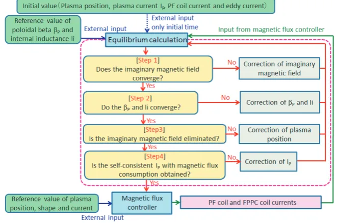
The plasma equilibrium control simulator consists of an equilibrium calculation component and a controller component. A function that calculates the self-consistentIP with flux consumption has been incorporated into the equilibrium calculation component in order to simulateIP
control. Figure 1 shows the calculation flow of the plasma equilibrium control simulator. In the equilibrium calcu-lation component of the simulator, the plasma position, shape andIPare obtained as a result of an equilibrium cal-culation. There are 4 calculation steps in the equilibrium calculation. Step 1, Step 2 and Step 3 were established in the previous plasma position and shape control simula-tor, and Step 4 has been added for the control ofIP. After finishing the calculation from Steps 1 to 3, the plasma po-sition and shape are obtained under the given coil current. At Step 4, the self-consistentIPwith flux consumption is
calculated in reference to the equilibrium obtained from
c
2013 The Japan Society of Plasma
Fig. 1 Calculation flow of the control simulator. It consists of an equilibrium calculation component and a controller component.
Step 1 to 3.
The function that controls theIPhas been incorporated
into the controller component in order to simulateIP
con-trol. The controller receives the reference values and ac-tual values of plasma position, shape, andIP. It modifies
the PF and FPPC coil currents to reduce the difference be-tween the reference values and actual values. At the next time step, the equilibrium calculation receives the modified coil current and reference values of the poloidal betaβP
and internal inductanceli. By iterating these procedures, feedback control of plasma position, shape, andIPby con-trolling the coil current is simulated.
2.1
Calculation of
I
Pwith flux consumption
TheIPwith the flux consumption is calculated at Step 4 in Fig. 1. The magnetic fluxΨop required for the
induc-tive operation is defined by:
Ψop=Ψramp+Ψflat-top, (1)
whereΨrampis the magnetic flux required for theIP
ramp-up, andΨflat-topis the magnetic flux required for the current
drive by inductive operation. The units of the variables
Ψop,Ψramp, andΨflat-topare in webers (Wb). TheIP
ramp-up is provided by the magnetic flux swing of the CS coils. The requiredΨrampis defined by:
Ψramp=LPIP+CEjimaμ0RPIP, (2)
whereLP is the plasma self-inductance, IP is the plasma current,RPis the plasma major radius,CEjima (=0.45) is the Ejima coefficient, andμ0 is the permeability of
vac-uum. Here the first and second terms on the right-hand side show the inductive and resistive flux consumption, re-spectively. The resistive flux consumption is calculated by the empirical Ejima formula forIPramp-up and from an
approximated loop voltage formula for flat-top. However, the requiredΨflat-topis defined by:
Ψflat-top=Vlooptflat-top, (3)
whereVloopis the approximated loop voltage, andtflat-topis the operation time. The relationship that indicates the flux balance is given by:
ΨInt−Ψop=ΨLink, (4)
whereΨInt andΨLink are the initial exciting flux and the
linked flux between the coils and the plasma, respectively. TheΨInt is constant, and the ΨLink is calculated by
inte-grating the flux generated by the PF coil and conducting elements. Substituting Eqs. (2) and (3) into Eq. (4), Eq. (4) can be rewritten as:
ΨInt−
LPIP+CEjimaμ0RPIP+Ψflat-top
=ΨLink;
(5) we then obtain:
Ψflat-top=ΨInt−
LPIP+CEjimaμ0RPIP+ΨLink
. (6) TheΨflat-top input, which indicates the input value of the
re-sistive flux for flat-top, is calculated using Eq. (3). Here, theIP, in which theΨflat-topcoincides with theΨflat-top input,
would be calculated by iteration. The correction of theIP
is given by:
dIP=
Ψflat-top−Ψflat-top input
LP+CEjimaμ0RP
, (7)
where dIPis the correction ofIP. The iteration of Step 4 is
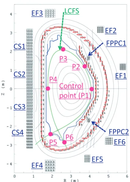
Fig. 2 Locations of the control points, the PF coils, in-vessel coils, and toroidal conducting elements in JT-60SA.
2.2
I
Pcontrol
The isoflux technique is used to control the position, shape, andIPin JT-60SA. The set of locations that defines the desired plasma separatrix is specified as the control points. Figure 2 shows the locations of the control points, PF coils, in-vessel coils, and toroidal conducting elements in JT-60SA.
The PF coil currents are adjusted to maintain an equal poloidal flux at the control points for the control of plasma position and shape. The small difference between the flux at the control points and its reference value is defined as δΨS. The change in the coil currents required for the
control of plasma position and shape is defined as dIC,PS. The relationship between dIC,PSandδΨSfor the control of
plasma position and shape can be represented as:
dIC,PS=GSM−1{δΨS}dt, (8)
whereM−1 is the (m×(n+1)) control matrix that is the generalized inverse of the Green functionMcalculated us-ing the sus-ingular value decomposition method, and m and n are the number of PF coils and control points, respec-tively. The matrix M−1 is used not only to control posi-tion and shape but also forIPcontrol. The Green function M represents the poloidal flux at the X/limiter point and each control point per unit of current. It is necessary to include the component of the X/limiter point in the matrix because the controller changes the poloidal flux equally at
the X/limiter point and control points forIPcontrol. GSis
the control gain of the position and shape feedback con-trols that are necessary to make the poloidal flux equal at all control points.
TheδΨSis defined as:
{δΨS}= ⎛ ⎜⎜⎜⎜⎜ ⎜⎜⎜⎜⎜ ⎜⎜⎜⎜⎝
0
Ψsurf−ΨP1
:
Ψsurf−ΨPn
⎞ ⎟⎟⎟⎟⎟ ⎟⎟⎟⎟⎟
⎟⎟⎟⎟⎠, (9)
whereδΨSis the (n+1) vector of the difference between
the reference flux value and the flux at the X/limiter point and control points,Ψsurf is the flux at the plasma surface,
andΨPn is the flux at the control point. It is necessary
to include the component of the X/limiter point inδΨSto
multiplyδΨSby the matrixM−1. The first element is the
difference at the the X/limiter point, and elements from the 2nd to the (n+1) rows are difference at the control points. Thus, the 1st row ofδΨSis zero. The units of the variables
are as follows: dIC is in amperes,GS is in s−1, andΨsurf
andΨPnare in webers.
However, the controller changes the poloidal flux equally at the X/limiter point and control points to reduce the difference between the actual value of IPand its ref-erence value without a change in the plasma position and shape forIPcontrol. The change in the poloidal flux re-quired forIPcontrol is defined as dΨsurf. The change in the
coil currents required forIPcontrol is defined as dIC,C. The
relationship between dIC,Cand dΨsurfforIPcontrol can be
presented as:
dIC,C=GCM−1{I}dΨsurf, (10)
whereGCis the control gain, andIis the (n+1) vector in which all elements are 1. The dΨsurf would be provided by
the PF coils in proportion to the difference between actual value ofIPand its reference value. Since the temporal dif-ferentiation of dΨsurf indicates the loop voltage, it can be
presented as:
Vloop=−dΨsurf
dt =Gr
IP,ref−IP, (11)
whereIP,refis the reference value ofIP, andGris the control gain. Therefore, Eq. (10) can be rewritten as:
dIC,C=−GCM−1{I}Grdt(IP,ref−IP). (12)
By definingGXasGCGrdt, Eq. (12) can be rewritten as:
dIC,C=−GXM−1{I}(IP,ref−IP), (13)
whereGX is the control gain of theIP feedback controls that are necessary to change the poloidal flux equally at all control points. Grdt is equal to LP from the equation of magnetic energy balance at the plasma surface.
modifies the PF coil currents according to the following equation:
IC(t+ Δt) = IC(t0)+M−1
GSP{δΨS(t)}
+GSI t
t0
{δΨS(t)}dt−GXP{I}(IP,ref−IP)
−GXI{I} t
t0
{IP,ref−IP}dt, (14)
wheret0 is the initial time; Δt is the control cycle; GSP
andGSI are the respective control gains of the P-I
feed-back controls that are necessary to make the poloidal flux equal at all control points; andGXPandGXIare the respec-tive control gains of the P-I feedback controls necessary to change the poloidal flux equally at all control points. The units of the variables are as follows:GSPandGXP are di-mensionless, andGSI andGXI are in s−1. The values of
GSP,GXP,GSI, andGXIare 1.0, 9.0, 1.0, and 10.0 in the following simulations, respectively.
3. Simulation Results
An operation scenario withIP ramp-up and pressure increase is developed using the plasma equilibrium con-trol simulator in JT-60SA. Equilibrium concon-trol capability against change in flux consumption is also to be discussed.
3.1
Study of the operation scenario during
I
Pramp-up
The control of plasma position, shape, andIPhas been simulated duringIP ramp-up. The controlled plasma pa-rameters are as follows: IPincreases from 1.0 to 5.5 MA, βPincreases from 0.10 to 0.74, andlidecreases from 0.84
to 0.74. The reference values ofIP,βP, andlichanges
dur-ingIPramp-up, and theIPprofile parameters are adjusted
to fix theβPandli to its reference value. All the
equilib-rium calculation cycles and control cycles of the PF coils and FPPC coils are 5 ms. Equilibrium control is simulated fromt = 2.7 to 25.0 s. The initial controlled plasma is
IP = 1.0 MA, βP =0.10, and li = 0.84 with the limiter
configuration. To make the transition from a limiter to a divertor configuration aroundt = 4.6 s,IP is maintained fromt=3.9 to 4.6 s.
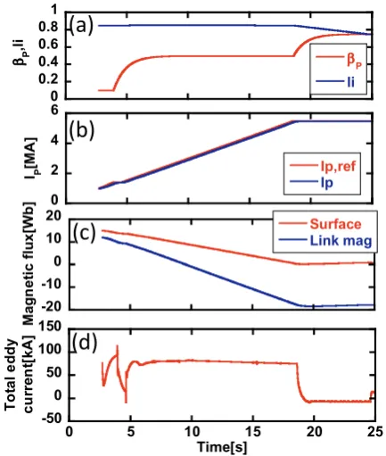
Figure 3 shows the waveforms of the plasma param-eters and total eddy current flowing in the conducting el-ements duringIPramp-up. TheβP andli are fixed to the
reference values as shown in Fig. 3 (a). The actual value of
IPincreases following the change in the reference value as shown in Fig. 3 (b). To do this, the poloidal flux at plasma surface and the linked flux increases (in the negative di-rection) duringIPramp-up as shown in Fig. 3 (c). The to-tal flux consumption calculated by the resistive and con-ductive consumption is in close agreement with the linked flux. The controller changes the poloidal flux equally at all control points, and the equilibrium calculation obtains theIPwith the flux consumption accurately. The total eddy
current flowing in the conducting elements is about 80 kA
Fig. 3 Simulation results duringIPramp-up. Waveforms of (a) the actual value ofβPandli, (b) the reference and actual values, (c) the flux at plasma surface and the linked flux between the plasma and coils, and (d) total eddy current flowing in the conducting elements.
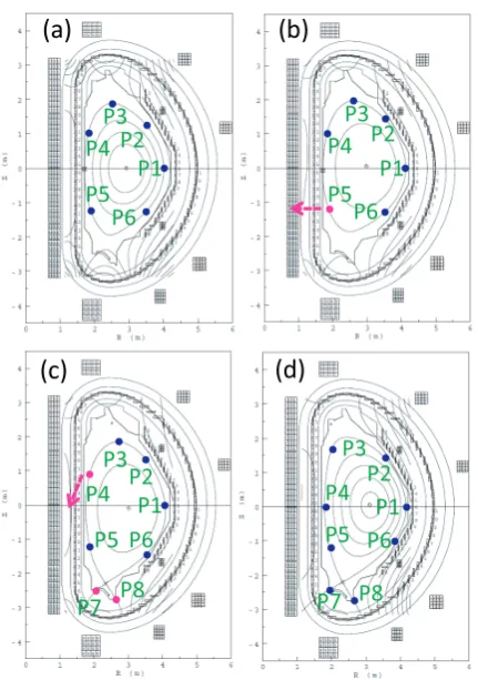
duringIPramp-up due to the change inIPand PF coil cur-rents. Figure 4 shows the equilibrium configurations at each time slice. The 6 initial input control points (P1 -P6) serves as the references for the plasma position and shape control att = 2.7 s. The transition from a limiter
to a divertor configuration is made in two steps: (1) an in-crease in the elongation, and (2) formation of the X point. Points P5 and P6 are moved in the horizontal and verti-cal directions, respectively, fromt = 3.9 to 4.6 s. As a result, the elongation increases from approximately 1.58 to 1.73 as the plasma shape changed to follow the control points. Points P7 and P8 are added to specify the location of the strike points att =3.905 s. The divertor
configura-tion is achieved by the formaconfigura-tion of the X point att=4.6 s.
The capability for the early formation of a divertor config-uration is preferable. After the transition to the divertor configuration, the Points P1–P6 are operated to increase the plasma volume. Finally, the elongation and triangular-ity become approximately 1.79 and 0.50, respectively, at
t =24.6 s. Figure 5 shows the waveforms of the residual
between the last closed flux surface (LCFS) and the con-trol points, and PF coil currents. The residual in the posi-tive direction indicates that the LCFS is outside the control point. The residual of P1, P2, and P6 initially increases by up to approximately 0.03 m due to an increase in both of theIPandβPas shown in Figs. 5 (a) and (b). The currents
Fig. 4 Simulation results duringIPramp-up. Equilibrium con-figurations (a) att = 2.7 s, (b) 3.9 s, (c) 4.6 s, and (d)
24.6 s.
Fig. 5 Simulation results during IP ramp-up. Waveforms of (a) residuals between P1-P3 and LCFS, (b) residuals be-tween P4 - P6, (c) coil currents of CS1 - CS4, and (d) coil currents of EF1 - EF6.
outer plasma surface inward to the control points as shown in Fig. 5 (d). At the same time, the currents of CS1 - CS4 increased (in the negative direction) to change the poloidal flux equally at all control points for theIPcontrol as shown
in Fig. 5 (c). Therefore, the simultaneous control of plasma
Fig. 6 Simulation results duringIPflat-top. Waveforms of (a) magnetic flux at the plasma surface and (b) coil currents of PF coils att=30.0 and 147.55 s.
position, shape, andIPis achieved duringIPramp-up.
3.2
Validation of the controllability of the
LCFS during
I
Pflat-top
The control of plasma position, shape, andIPhas been simulated to validate the controllability of the LCFS dur-ing IP flat-top. The PF coils need to keep changing the poloidal flux equally at all control points to maintain the
IPfor the inductive operation. However, it is known how difficult it is to keep the desired plasma shape by maintain-ingIPfor a long time because changing the coil current of
the finite length CS modules distorts the actual magnetic field around upper and lower sides of the plasma. The first example of validating the controllability of the LCFS is discussed with the change in PF coil currents for a long time. The controlled plasma parameters are as follows:
IP = 5.5 MA,βP = 0.74, and li = 0.74 with the divertor
configuration. All the equilibrium calculation cycles and the control cycles of the PF coils are 5 ms. The simulation should be performed until the PF coil achieves the limit of coil current in order to validate the controllability of the LCFS for as long as possible. The limit of PF coil cur-rents are±20 kA. The 8 initial input control points (P1 -P8) serve as the references for the position and shape. The location of the control points are fixed at the initial loca-tion. Figure 6 show the waveforms of the poloidal flux at the plasma surface and the currents of PF coils. The currents of CS1 - CS4 increase (in the negative direction) to maintain theIPfor the inductive operation as shown in Fig. 6 (b). The current of CS2 reaches the limit of coil cur-rent att = 147.55 s. The loop voltage is given as 0.06 V
duringIPflat-top. The controller changes the poloidal flux
by about 7.044 Wb fromt = 30.0 to 147.55 s. The
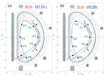
Fig. 7 Simulation results duringIPflat-top. (a) LCFS without optimizing the location of P3 att=30.0 (red solid line) and 147.55 s (blue solid line), and (b) LCFS with opti-mizing the location of P3 att=30.0 (red solid line) and 145.89 s (blue solid line).
induced by the change of the currents in CS1 and CS4. The effect of changing the current in PF coil on the controlla-bility of the LCFS has been validated by the comparison of the LCFS att = 30.0 s and the ending time when the
limit of currents of CS coil is reached. Figure 7 (a) shows the comparison of the LCFS att=30.0 and 147.55 s. The
location of the control points is fixed based on the above operation scenario duringIPramp-up. Though the residual of the control points is almost zero, the difference in the LCFS around the upper and lower sides is observed over time. The location ofZtop, which is the top of the LCFS, increases from 2.117 to 2.196 m, and thus the elongation also increased from 1.827 to 1.864. The changing currents in the PF coils cause an unexpected change in the LCFS. This unexpected change in the LCFS has the potential to destabilize the control. To maintain the controllability of the LCFS during IP flat-top, the location of the control
point is optimized. Figure 7 (b) shows the comparison of the LCFS att=30.0 and 145.89 s. The location of control
point P3 is optimized to control the LCFS duringIP flat-top. The difference in the LCFS decreases near the upper side, and thus the change in the location ofZtop and elon-gation are controlled. The location of control point also should be optimized to maintain the controllability of the LCFS duringIPflat-top.
4. Summary
A plasma equilibrium control simulator was devel-oped for exploration of techniques to control plasma posi-tion, shape, andIP. Functions to calculate and control the
IPwith flux consumption were incorporated in the plasma position and shape control simulator. It is possible to simu-late the control of the position, shape, andIPand optimize the control logic in JT-60SA.
The control of plasma position, shape, andIPhas been simulated duringIP ramp-up. The actual value of IP in-creased to follow the change in the reference value. The di-vertor configuration is achieved with the formation of an X point at the reference time by operating the control points. The simultaneous control of plasma position, shape, andIP
is achieved duringIPramp-up.
The control of plasma position, shape, andIPhas been
simulated to validate the controllability of the LCFS dur-ingIP flat-top. The PF coil current needs to be changed
continuously in order to control the poloidal flux equally at all control points to maintain theIPfor inductive
oper-ation. The change of currents in the PF coils causes an unexpected change in the LCFS. The location of control point also should be optimized to maintain the controlla-bility of the LCFS duringIPflat-top.
In the future, the simulator will incorporate a coil voltage control scheme and plasma boundary identification code. Currently, the control points are manually adjusted to control the plasma position and shape. The new system will incorporate a control interface that will automatically adjust the number and location of control points in refer-ence to the given plasma shape parameters such as elon-gation and triangularity. The controllability of the vertical instability will be validated using the simulator.
[1] S. Ishidaet al., Fusion Eng. Des.85, 2070 (2010). [2] Y. Kamadaet al., Nucl. Fusion51, 073011 (2011). [3] K. Tobitaet al., Fusion Eng. Des.81, 1151 (2006). [4] K. Tobitaet al., Nucl. Fusion49, 075029 (2009).
[5] R.R. Khayrutdinov et al., J. Comput. Phys. 107, 106 (1993).