Intertemporal Changes in Risk Dynamics of
Different Types of Banks
Semen SON-TURAN
MEF University, Faculty of Economics, Administrative and Social Sciences, Istanbul, Turkey
Abstract
This original study compares two groups of banks operating in the same market in Turkey to determine differences in underlying risk dynamics of Islamic banking stocks. To that end, event-related ARCH family models and in-sample and out-of-in-sample forecasts are applied, where two Turkish general election dates (06/12/2011 and 6/7/2015) serve as cut-off points of the sub-samples. The rationale for using general election dates to determine sub-periods is to understand whether there is a noticeable change of reaction of Islamic banking stocks, in particular, that influences mean returns and conditional volatility, and, whether or not, the models’ forecasting accuracy changes over time. Results indicate the presence of intertemporal changes in risk dynamics among the two groups of banks.
Keyword: Stock return volatility, volatility forecasting, GARCH, EGARCH, mixture of distributions
JEL Classification: G02, G10, G14, G17
1.INTRODUCTION
Islamic finance and Islamic banking are concepts that emerged in the 1970s with the inception of the Islamic banking industry. Following the establishment of the Dubai Islamic Bank in 1975, many banking institutions operating on the principles of Islam propagated (Cox, 2002). Many countries today have a dual banking system, in which there are Islamic banks alongside traditional banks. Islamic banking operates according to the principles of the Islamic code of law and behavior (sharia) based on the Quran, prohibits paying and receiving interest (riba) and leaves no room for speculation or uncertainty (gharar). Along these lines money is considered to be solely a medium of exchange.
In Turkey there are currently four Islamic or so-called “participation” banks that follow Islamic principles: Albaraka Türk, Bank Asya, Kuveyt Türk and Türkiye Finans. Together these banks hold assets of a size of TRL 104,242 mn as of 2014 December that amounts to 5.2% in relation to the total assets in the Turkish banking industry. In terms of funds allocated and funds collected, these percentages are 5.4% and 6.2%, respectively. However, only two of these banks’ shares are quoted on the Borsa Istanbul Stock Exchange („BIST”). Furthermore, on September 30, 2014, Bank Asya shares were moved to the BIST watchlist companies market, where companies are kept under surveillance.
This paper aims at understanding whether and/or how the riskiness of the two different types of banking stocks operating in the Turkish equity market changes according to sub-periods.
In particular this study, firstly seeks to determine which of the most frequently used symmetric and asymmetric ARCH-family models in an event-study context, best explain the heteroskedasticity inherent in the OLS residuals of Islamic and conventional banks’ stock returns, and, whether, through the inclusion of regressors such as dividend yield and trading volume as substantiated by respective literature resting on the Mixture of Distribution Hypothesis (Clark, 1973; Epps and Epps,1976; Lamoureux and Lastrapes, 1990) and Efficient Markets Hypothesis (Fama,1965), nested versions of such models should be preferred as risk management tools on the basis that they potentially are better fitting models and/or reduce volatility persistence relatively more than their alternatives. Secondly, subsequent to in-sample forecasts, out-of-sample forecasts are conducted, where two Turkish general election dates (06/12/2011 and 6/7/2015) serve as cut-off points of sub-samples. The rationale for using general election dates to determine sub-periods is to understand whether there is a noticeable change of reaction of Islamic banking stocks, in specific, that influences mean returns and conditional volatility and, whether or not, the models’ forecasting accuracy changes over time. Lastly, one-step-ahead forecasts are conducted and the forecasting performance of the models are compared.
*
Corresponding Author, Department of Business Administration, MEF University, Turkey, E-mail: [email protected]
2. LITERATURE REVIEW
Some researchers view Islamic financial institutions as a viable alternative to promote economic growth and think they are better-suited to absorb macro-financial shocks due to structural advantages over conventional banks (Dridi and Hasan, 2010; Ebrahim and Safadi, 1995; Mills and Presley, 1999). On the other hand, studies exist that argue that the recent financial crisis led to difficulties in many conventional banks across the globe but that Islamic banks were largely insulated from the crisis (Willison, 2009; Yılmaz, 2009). Furthermore, other studies (El-Gamal, 2005), in contrast, argue that Islamic finance simply seeks to replicate the functions of conventional financial instruments and in that sense is a form of rent-seeking legal arbitrage.
Considering their increasing importance, the lack of studies on the subject of Islamic financial markets brings out the necessity for a thorough understanding of the efficiency in Islamic equity markets.
The more recent strand of literature investigates the links between Islamic and conventional financial markets in terms of relative return and volatility. It also focuses on the relative performance between these markets during the recent global financial crisis (Ajmi et al., 2014). Although the risk-return performances of Islamic and conventional equity markets have been compared frequently, the number of studies comparing their market efficiency is fairly low. In fact, except the recent works by Alvarez-Diaz et al. (2014) and Khalichi et al. (2014), no solid studies have performed a comparative efficiency analysis on Islamic and conventional equity markets, moreover their results seem to contradict with each other.
Gupta et al. (2014) use a wide variety of linear and non-linear predictive regression models, based on a large number of predictors, to indicate that these models cannot outperform the (benchmark) autoregressive model in forecasting the Dow Jones Islamic Market Index (DJIM) returns. Authors state that the prohibition of interest rates in the Islamic finance industry possibly shuts off the channels that connect market returns with economic activity, which in turn complicates the attempts to forecast the Islamic stock returns.
3. METHODOLOGY AND DATA
Since it is expected that conventional and Islamic banks’ stocks volatility behavior changes with respect to the sub-period and, furthermore, that Islamic equity markets are less efficient and thus should display discernible patterns, an autoregressive term in the mean equation and leverage effect in the conditional volatility equation are probable. Thus the first hypothesis becomes:
H1a: Heteroskedasticity in OLS residuals of Islamic banks’ stock returns is best explained by AR(1)-EGARCH(1,1)
In contrast, conventional banks’ stocks that appeal to a relatively diverse audience of investors are more prone to forming an informationally efficient market, with a decreased probability of a pattern in stock price formation. Furthermore, in accordance with various studies resting on the Mixture of Distributions Hypothesis trading volume is frequently found to be a significant regressor in the conditional variance equation. Thus, the second hypothesis becomes:
H1b: Heteroskedasticity in OLS residuals of conventional banks’ stock returns residuals is best explained by MM-GARCH(1,1)-V
Finally, the author expects that the two elections of 2011 and 2015 in Turkey, which resulted in a majority government and a (second) subsequent election, respectively, produce different investor sentiment and hence, affect the forecast accuracy of the model. Accordingly, the last hypothesis is formulated as follows:
H2: The forecast accuracy of respective models w.r.t. stock returns and conditional volatility changes according to sub-periods.
The data is composed of the observed series of stock prices over the period from June 20, 2008 - June 19, 2015 and is collected on a daily basis amounting to a total of 1826 trading days.
The sample consists of two Turkish Islamic banks and three conventional banks and the BIST Banking Index that are traded on the Borsa Istanbul Stock Exchange. All data is obtained from Data Stream.
The criteria for sample selection for conventional banks are their asset sizes that are comparable to the participation banks’ asset sizes. İş Bank was included representing one of the largest and oldest banks in Turkey. The closest benchmarks (i.t.o. asset size) to ATB and ASA are SEK and TSK respectively.
rt = ln Pt – ln Pt-1 (1)
Respective Augmented Dickey Fuller tests are applied to test for stationarity.
Table 1: Total Asset Sizes (31.12.2014) of Banks
Name Symbol Date of Establishment Total Assets
Conventional Banks
Turkiye Is Bankası A.S. ISCTR 1924 237,772
Sekerbank T.A.S. SKBNK 1953 21,187
Türkiye Sinai Kalkinma Bankasi A.S. TSKB 1950 15,701
Participation Banks
AlbarakaTurk ALBRK 1984 23,046
Bank Asya ASYAB 1996 13,680
Source: Author’s own elobaroation based on data from TBB and TKBB
Prior to modelling, OLS residuals are tested for heteroskedasticity, autocorrelation and normality. Following diagnostic testing, mean specifications AR(1) and the basic market model (MM) are used in combination with GARCH(1,1) and EGARCH(1,1) as conditional variance specifications. Also nested versions of the conditional variance specifications where dividend yield and trading volume are added as regressors in a step-wise manner are tested. AR(1) and the basic market model (MM) mean specifications in combination with GARCH(1,1) and EGARCH(1,1) conditional variance specifications, and increasingly nested versions of such, are applied. Subsequently, all model residuals undergo residual diagnostic testing to determine whether any ARCH effect or serial correlation is left in the residuals.
The mean specifications that are being tested are:
The GARCH (p,q) that is used to model the conditional variance has two characteristic parameters: the number of GARCH terms defined by p referring to the number of autoregressive lags and the number of ARCH terms defined by q referring to the number of moving average lags.
Equation (5) depicts a GARCH(1,1) model where there is a constant (), an ARCH term ( 2
1 1
t
) at first lag anda GARCH ( 2
1 t
) term at first lag, with positivity constraints for > 0, and parameters 1 0, 1 > 0, and1 + 1 <1.
The GARCH (1,1) model solves for the conditional variance as a function of its previous variance, its previous squared return and the long-run variance. The sum of the ARCH and GARCH term parameters is called volatility persistence and refers to how quickly the variance reverts or “decays” toward its long-run average. If persistence is high (low), this means that the decay and the reversion to the mean is slow (quick). If the sum of
2 1 1 2
1 1 2
t t
t
(5)The market model,
rt = c+ λ1M + ε (2)
and,
The AR(1) market model
rt = c+ rt-1 + λ1M + ε (3)
Where r, M, rt-1 stand for expected return, market return and lagged return, respectively.
The variance specification for the GARCH(1,1) is:
ARCH () and GARCH () parameters is 1, this implies there is no mean reversion. If persistence is less than 1, this means there is a reversion to the mean. If persistence is low, this implies a greater reversion to the mean. The variance specification for the EGARCH(1,1) is:
)
log(
)
log(
211 1
1 1 2
tt t
t t
t
(6)ARCH and GARCH models assume that volatility is inherently symmetric. However, under the Value Function property proposed by Kahneman and Tversky (1979), investors react asymmetrically to good versus bad news. This asymmetric response is adressed by the EGARCH model of Nelson (1991), as illustrated in equation (6): Since the left-handside of the equation is the logarithm of the conditional variance, the positivity
constraints imposed upon the model parameters by GARCH are lifted in the EGARCH model. Here,
1 1
t t
is the
leverage effect, occuring when
<0 (positive news generate less volatility than negative ones), that seeks tocapture impacts of positive and negative news shocks on volatility. Asymmetry is present when
0
meaningthat the market differentiates between positive and negative news.
Asymmetric response is often time described with the “leverage or bad news effect” first presented by Black (1976). A drop in the value of a stock (negative return) increases the financial leverage; this makes the stock riskier and thus increases its volatility. Therefore if we were to price volatility, an expected increase in volatility would raise the required return on equity.
Recalling the Value Function property of Prospect Theory, which simply states that individuals assign more value to losses rather than gains, we can argue that the EGARCH takes account of this very same behavioral phenomenon through adding the “bad news” component to its model.
Modelling is applied to two sub-periods, where the rationale for the cut-off dates are determined by the Turkish general election dates.
Thus, the modelling is performed on the hold-out sample and validation on the remainder of the data. Thus in-sample and out-of-sample forecasts are applied to each sub-period. Table 2 presents the sub-periods.
The model is composed of two parts (estimation and validation) thus, there are two periods marked by the cut-off dates of general elections, which are 06/12/2011 and 06/07/2015.
Table 2: Sub-Periods
Estimation (in-sample)
Validation (out-of-sample)
Forecasting (1-step ahead)
1st sample 06/20/2008-06/10/2011 06/13/2011- 06/19/2015 06/22/2015
2nd sample 06/13/2011-06/05/2015 06/08/2015-06/19/2015 06/22/2015
4. RESULTS
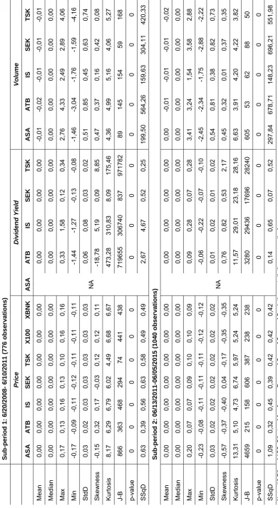
Table 3: Des criptiv e Statistics Su b -p e rio d 1: 6/20/20 08- 6/1 0 /201 1 (77 6 o b ser v a tio n s ) Pric e Div ide nd Yie ld Volume A S A A T B IS SEK TSK X100 XBNK A S A A T B IS SEK TSK A S A A T B IS SEK TSK Mean 0,00 0,00 0,00 0,00 0,00 0,00 0,00 NA 0,00 0,00 0,00 0,00 -0,01 -0,02 -0,01 -0,01 -0,01 Medi an 0,00 0,00 0,00 0,00 0,00 0,00 0,00 0, 00 0,00 0,00 0,00 0,00 0,00 0,00 0,00 0,00 Max 0,17 0,13 0,16 0,13 0,10 0,16 0,16 0,33 1,58 0,12 0,34 2,76 4, 33 2,49 2,89 4,06 Min -0,17 -0,09 -0 ,11 -0,12 -0,11 -0 ,11 -0,11 -1,44 -1,27 -0,13 -0,0 8 -1 ,4 6 -3 ,0 4 -1 ,7 6 -1 ,5 9 -4 ,1 6 StdD 0,03 0,02 0,03 0, 03 0,03 0,03 0,03 0,06 0,08 0,03 0,02 0,51 0,85 0,45 0,63 0,74 Ske w ne ss -0,15 0,32 0,17 -0,03 0,12 0,12 0,11 -18,78 5,19 0,09 8,85 0,47 0,37 0,16 0,42 0,08 Kurtosis 8,17 6,29 6,79 6,02 4,49 6,68 6,67 473,2 8 310,8 3 8,09 175,4 6 4,36 4, 99 5,16 4,06 5,27 J-B 866 363 468 294 74 441 438 719 65 5 306 74 0 837 971 78 2 89 145 154 59 168 p-val ue 0 0 0 0 0 0 0 0 0 0 0 0 0 0 0 0 SSqD 0,63 0,39 0,56 0,63 0,58 0,49 0,49 2,67 4,67 0,52 0,25 199,5 0 564,2 6 159,6 3 304,1 1 420,3 3 Su b -p e rio d 2: 06/13/2 0 1 1 -06/ 05/20 15 (1 040 o b ser v a tio n s ) Mean 0,00 0,00 0,00 0,00 0,00 0,00 0,00 NA 0,00 0,00 0,00 0,00 0,00 -0,01 -0,01 -0,01 -0,02 Medi an 0,00 0,00 0,00 0,00 0,00 0,00 0,00 0, 00 0,00 0,00 0,00 0,00 0,00 0,00 0,00 0,00 Max 0,20 0,07 0,07 0,09 0,10 0,10 0,09 0,09 0,28 0,07 0,28 3,41 3, 24 1,54 3,58 2,88 Min -0,23 -0,08 -0 ,11 -0,11 -0,11 -0 ,12 -0,12 -0,06 -0,22 -0,07 -0,1 0 -2 ,4 5 -2 ,3 4 -1 ,7 5 -2 ,8 8 -2 ,2 2 StdD 0,03 0,02 0,02 0, 02 0,02 0,02 0,02 0,01 0,02 0,01 0,02 0,54 0,81 0,38 0,82 0,73 Ske w ne ss -0 ,5 7 -0 ,3 7 -0 ,4 0 0,0 4 -0 ,1 7 -0 ,3 5 -0 ,3 5 0, 76 0,82 0,53 2,17 0,45 0,32 0,01 0,37 0,35 Kurtosis 13,31 5,10 4,73 6,74 5, 97 5,24 5,24 11,57 29, 01 23,18 28,16 6,63 3, 91 4,20 4,22 3,82 J-B 465 9 215 158 606 387 238 238 328 0 294 36 176 96 282 40 605 53 62 88 50 p-val ue 0 0 0 0 0 0 0 0 0 0 0 0 0 0 0 0 SSqD 1,09 0,32 0,45 0,39 0,42 0,42 0,42 0,14 0,65 0,07 0,52 297,8 4 678,7 1 148,2 3 696,2 1 551,9 8 Note
: “J-B” a
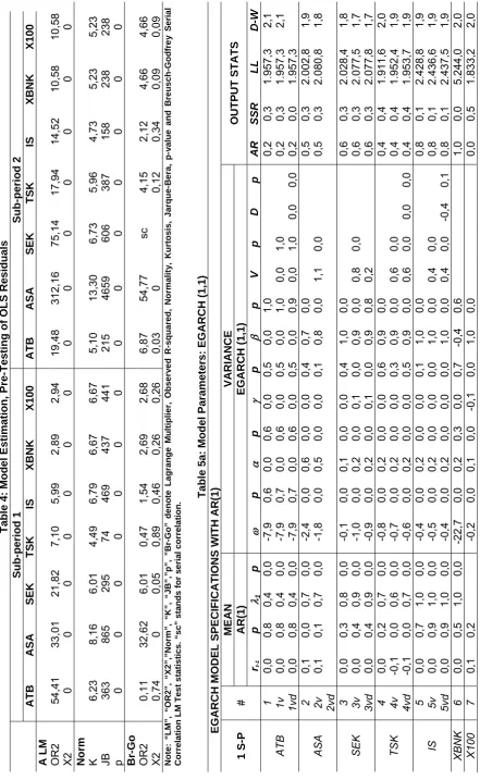
Table 4: Mod
e
l Estimatio
n, Pre-Tes
tin
g of OLS Re
siduals Sub-period 1 Sub-period 2 A T B A SA SEK TSK IS XB NK X100 A T B A SA SEK TSK IS XB NK X100 A LM OR2 54,41 33,01 21,82 7,10 5,99 2,89 2,94 19,48 312,16 75,14 17,94 14,52 10,58 10,58 X2 0 0 0 0 0 0 0 0 0 0 0 0 0 0 Norm K 6,23 8,16 6,01 4,49 6,79 6,67 6,67 5,10 13,30 6,73 5,96 4,73 5,23 5,23 JB 363 865 295 74 469 437 441 215 4659 606 387 158 238 238 p 0 0 0 0 0 0 0 0 0 0 0 0 0 0 Br-G o OR2 0,11 32,62 6,01 0,47 1,54 2,69 2,68 6,87 54,77 sc 4,15 2,12 4,66 4,66 X2 0,74 0 0,05 0,89 0,46 0,26 0, 26 0,03 0 0,12 0,34 0,09 0,09 No te : “L
M”, “OR2”, “X2”,”No
rm
”, “K”, “JB”,”p
” , ”Br-Go ” d e n o te L a g ran ge Multipl ier, Obse rv e d R-sq uared , Norm alit y , Ku rtosis, J ar qu e-Bera, p -v a lue a nd Bre u sc h-Go dfre y Seria l Correlati
on LM Test
s
tatis
tics. “sc”
stands for serial
correla
tio
n
. Table 5a
: Mo
del Parameters: EG
ARCH (1,1 ) EGARCH MODEL SPECI F ICATIONS WITH AR(1) 1 S-P # MEAN VARIA N C E OUTP UT ST ATS AR (1 ) EGAR C H (1, 1) rt-1 p 1 p p p p
p V p
EGARCH MODEL SPECI
F
ICATIONS
WITH
AR(1)
2 S-P
#
MEAN
VARIANCE
OUTP
UT
STATS
AR(1)
EGARCH
(1,
1)
rt-1
p
1
p
p
p
p
p V
p
D
p
AR
SSR
LL
D-W
ATB
1
0,0
0,4
0,5
0,0
-1,2
0,0
0,2
0,0
-0,1
0,0
0,9
0,0
0,3
0,2
2.974,6
2,0
1v
-0,1
0,0
0,4
0,0
-1,3
0,0
0,2
0,0
0,0
0,
0
0,9
0,0
0,6
0,0
0,3
0,2
3.020,7
1,9
1vd
-0,1
0,0
0,4
0,0
-1,3
0,0
0,2
0,0
0,0
0,1
0,9
0,0
0,6
0,0
0,7
0,
6
0,3
0,2
3.020,8
1,9
ASA
2
-0,1
0,1
0,7
0,0
-1,2
0,0
0,6
0,0
0,1
0,0
0,9
0,0
0,1
1,0
2.566,1
1,4
2v
-0,1
0,0
0,7
0,0
-0,8
0,0
0,5
0,0
0,1
0,
0
0,9
0,0
1,1
0,0
0,1
1,0
2.661,9
1,4
2vd
SEK
3
-0,1
0,1
0,4
0,0
-3,3
0,0
0,5
0,0
0,1
0,0
0,6
0,0
0,2
0,3
2.819,6
1,9
3v
-0,1
0,0
0,4
0,0
-1,7
0,0
0,4
0,0
0,1
0,
0
0,8
0,0
0,9
0,0
0,2
0,3
2.940,5
1,8
3vd
-0,1
0,0
0,4
0,0
-1,7
0,0
0,4
0,0
0,1
0,0
0,8
0,0
0,9
0,0
8,7
0,
1
0,2
0,3
2.943,4
1,8
TSK
4
-0,1
0,0
0,6
0,0
-3,7
0,0
0,2
0,0
-0,1
0,0
0,6
0,0
0,4
0,2
2.889,5
1,9
4v
-0,1
0,0
0,6
0,0
-3,1
0,0
0,3
0,0
-0,1
0,1
0,7
0,0
0,7
0,0
0,4
0,2
2.940,6
1,9
4vd
-0,1
0,0
0,6
0,0
-3,3
0,0
0,3
0,0
-0,1
0,0
0,6
0,0
0,7
0,0
-2,4
0,0
0,4
0,2
2.942,1
1,9
IS
5
0,0
0,9
1,0
0,0
-0,8
0,0
0,2
0,0
0,0
0,0
0,9
0,0
0,8
0,1
3.563,0
1,9
5v
0,0
0,6
1,0
0,0
-1,6
0,0
0,2
0,0
0,1
0,
0
0,8
0,0
1,0
0,0
0,8
0,1
3.605,6
2,0
5vd
0,0
0,6
1,0
0,0
-1,6
0,0
0,2
0,0
0,1
0,0
0,8
0,0
1,0
0,0
-1,9
0,0
0,8
0,1
3.607,6
2,0
XBNK
6
0,0
0,9
1,0
0,0
-11,4
0,7
0,0
0,8
0,0
0,8
0,3
0,9
1,0
0,0
7.024,8
2,0
X100
7
0,0
0,6
-
-0,6
0,0
0,2
0,0
-0,1
0,
0
0,9
0,0
0,0
0,4
2.620,8
2,1
EGARCH MODEL SPECI
F
ICATIONS
WITH MARKET MODEL
1 S-P
MEAN
VARIANCE
OUTP
UT
STATS
MM
EGARCH
(1,
1)
1
p
p
p
p
p
V
p D p
AR
SSR
LL
D-W
ATB
0,4
0,0
-3,2
0,0
0,5
0,0
0,0
0,2
0,6
0,0
0,2
0,3
1.999,9
2,1
0,4
0,0
-2,6
0,0
0,6
0,0
-0,1
0,0
0,
7
0,0
0,6
0,0
0,2
0,3
2.046,4
2,1
0,4
0,0
-3,5
0,0
0,6
0,0
-0,1
0,1
0,6
0,0
0,6
0,0
-4,8
0,0
0,2
0,3
2.055,7
2,1
ASA
0,7
0,0
-2,7
0,0
0,6
0,0
0,0
0,5
0,7
0,0
0,5
0,3
1.998,5
1,7
0,7
0,0
-1,8
0,0
0,5
0,0
0,0
0,1
0,
8
0,0
1,2
0,0
0,5
0,3
2.078,4
1,6
SEK
0,9
0,0
-0,1
0,0
0,1
0,0
0,0
0,3
1,0
0,0
0,6
0,3
2.028,0
1,8
0,9
0,0
0,2
0,0
0,1
0,0
0,9
0,0
0,
8
0,0
0,6
0,3
2.077,2
1,8
0,9
0,0
-0,9
0,0
0,2
0,0
0,1
0,0
0,9
0,0
0,8
0,0
0,7
0,2
0,6
0,3
2.077,6
1,8
TSK
0,7
0,0
-0,8
0,0
0,2
0,0
0,0
0,6
0,9
0,0
0,4
0,4
1.910,8
2,1
0,7
0,0
-0,7
0,0
0,2
0,0
0,0
0,3
0,
9
0,0
0,6
0,0
0,4
0,4
1.949,1
2,1
0,7
0,0
-0,6
0,0
0,2
0,0
0,0
0,6
0,9
0,0
0,6
0,0
2,4
0,0
0,4
0,4
1.950,6
2,1
IS
1,0
0,0
-0,4
0,0
0,2
0,0
0,0
0,0
1,0
0,0
0,8
0,1
2.428,8
1,9
1,0
0,0
-0,5
0,0
0,2
0,0
0,0
0,0
1,
0
0,0
0,4
0,0
0,8
0,1
2.436,6
1,9
1,0
0,0
-0,4
0,0
0,2
0,0
0,0
0,0
1,0
0,
0
0,4
0,0
-0,4
0,1
0,8
0,1
2.437,5
1,9
XBNK
1,0
0,0
-21,8
0,0
0,2
0,3
0,0
0,4
-0
,3
0,6
0,0
0,0
5.243,8
1,9
X100
-0,2
0,0
0,1
0,0
0,0
0,0
1,
0
0,0
0,0
0,5
1.832,3
1,9
EGARCH MODEL SPECI
F
ICATIONS
WITH MARKET MODEL
2 S-P
MEAN
VARIANCE
OUTP
UT
STATS
MM
EGARCH
(1,
1)
1
p
p
p
p
p V
p
D
p
AR
SSR
LL
D-W
ATB
0,5
0,0
-1,2
0,0
0,2
0,0
-0,1
0,0
0,9
0,0
0,3
0,2
2.974,2
2,0
0,4
0,0
-1,3
0,0
0,2
0,0
0,0
0,0
0,
9
0,0
0,5
0,0
0,3
0,2
3.017,6
2,0
0,5
0,0
-1,3
0,0
0,2
0,0
0,0
0,1
0,9
0,0
0,5
0,0
0,5
0,8
0,3
0,2
3.017,7
2,0
ASA
0,7
0,0
-1,2
0,0
0,6
0,0
0,1
0,0
0,9
0,0
0,1
0,9
2.565,2
1,5
0,7
0,0
-0,8
0,0
0,5
0,0
0,1
0,0
0,
9
0,0
1,0
0,0
0,1
0,9
2.657,6
1,5
SEK
0,4
0,0
-3,2
0,0
0,5
0,0
0,1
0,0
0,7
0,0
0,2
0,3
2.817,8
2,1
0,4
0,0
-1,7
0,0
0,4
0,0
0,1
0,0
0,
8
0,0
0,8
0,0
0,2
0,3
2.933,8
2,1
0,4
0,0
-1,8
0,0
0,4
0,0
0,1
0,0
0,8
0,0
0,8
0,0
8,7
0,1
0,2
0,3
2.936,7
2,1
TSK
0,6
0,0
-3,8
0,0
0,2
0,0
-0,1
0,0
0,6
0,0
0,4
0,2
2.887,5
2,1
0,6
0,0
-3,3
0,0
0,3
0,0
-0,1
0,1
0,
6
0,0
0,6
0,0
0,4
0,2
2.936,6
2,1
0,6
0,0
-3,5
0,0
0,3
0,0
-0,1
0,0
0,6
0,0
0,6
0,0
-2,5
0,0
0,4
0,2
2.938,2
2,1
IS
1,0
0,0
-0,8
0,0
0,2
0,0
0,0
0,0
0,9
0,0
0,8
0,1
3.563,0
2,0
1,0
0,0
-1,6
0,0
0,2
0,0
0,1
0,0
0,
8
0,0
1,0
0,0
0,8
0,1
3.605,5
2,0
1,0
0,0
-1,6
0,0
0,2
0,0
0,1
0,0
0,8
0,
0
1,0
0,0
-1,9
0,0
0,8
0,1
3.607,4
2,0
XBNK
1,0
0,0
-1,3
0,0
0,0
0,8
0,0
0,9
0,9
0,0
1,0
0,0
7.025,2
2,0
X100
-0,6
0,0
0,2
0,0
-0,1
0,0
0,
9
0,0
0,0
0,4
2.620,7
2,1
Table 5b: Mo
del Parameters: G
A
RCH(1,1)
GARCH MODEL SPECIFICATION WI
TH AR(1)
1 S-P
#
MEAN
VARIANCE
OUTP
UT
STATS
AR
(1
)
GAR
C
H
(1,1)
rt-1
p
1
p
p
p
p V
p
D
p
AR
SSR
LL
D-W
ATB
1
-0,02
0,60
0,40
0,00
0,00
0,00
0,31
0,00
0,41
0,00
0,25
0,29
1.998,39
2,05
1v
-0,03
0,60
0,38
0,00
0,00
0,00
0,27
0,00
0,39
0,00
0,00
0,02
0,24
0,30
2.022,65
2,03
1vd
-0,01
0,81
0,43
0,00
0,00
0,00
0,06
0,07
0,47
0,
01
0,00
0,00
0,00
0,00
0,24
0,30
1.982,68
2,05
ASA
2
0,12
0,01
0,69
0,00
0,00
0,00
0,41
0,00
0,44
0,00
0,51
0,31
2.002,61
1,89
2v
0,15
0,01
0,70
0,00
0,00
0,00
0,21
0,00
0,48
0,00
0,00
0,
00
0,51
0,31
2.033,37
1,94
2vd
SEK
3
0,03
0,30
0,85
0,00
0,00
0,01
0,02
0,00
0,97
0,00
0,58
0,27
2.028,44
1,83
3v
0,01
0,75
0,87
0,00
0,00
0,00
0,04
0,00
0,89
0,00
0,00
0,
00
0,57
0,27
2.061,82
1,79
3vd
0,01
0,75
0,86
0,00
0,00
0,00
0,
04
0,00
0,89
0,00
0,00
0,00
0,
00
0,60
0,57
0,27
2.061,89
1,79
TSK
4
-0,05
0,20
0,66
0,00
0,00
0,00
0,19
0,00
0,60
0,00
0,37
0,36
1.909,55
2,04
4v
-0,03
0,46
0,66
0,00
0,00
0,00
0,06
0,01
0,45
0,00
0,00
0,00
0,37
0,36
1.909,51
2,07
4vd
-0,03
0,40
0,66
0,00
0,00
0,00
0,06
0,00
0,45
0,
00
0,00
0,00
0,00
0,60
0,37
0,36
1.909,38
2,07
IS
5
0,02
0,63
0,97
0,00
0,00
0,01
0,10
0,00
0,87
0,00
0,82
0,10
2.427,92
1,89
5v
0,01
0,72
0,97
0,00
0,00
0,00
0,09
0,00
0,87
0,00
0,00
0,
00
0,82
0,10
2.435,12
1,88
5vd
0,01
0,80
0,97
0,00
0,00
0,00
0,
09
0,00
0,88
0,00
0,00
0,00
0,
00
0,00
0,82
0,10
2.437,57
1,88
XBNK
6
1,00
0,00
0,00
0,90
0,00
0,95
0,57
0,80
1,00
0,00
5.242,28
2,00
X100
7
0,04
0,35
-
0,00
0,03
0,07
0,00
0,92
0,00
0,00
0,49
1.829,30
1,96
GARCH MODEL SPECIFICATION WI
TH AR(1)
2 S-P
#
MEAN
VARIANCE
OUTP
UT
STATS
AR
(1
)
GAR
C
H
(1,1)
rt-1
p
1
p
p
p
p V
p
D
p
AR
SSR
LL
D-W
ATB
1
-0,03
0,32
0,47
0,00
0,00
0,00
0,11
0,00
0,74
0,00
0,33
0,21
2.971,67
1,97
1v
-0,06
0,09
0,46
0,00
0,00
0,00
0,12
0,00
0,68
0,00
0,00
0,00
0,33
0,21
3.007,19
1,92
1vd
-0,06
0,08
0,46
0,00
0,00
0,00
0,12
0,00
0,67
0,
00
0,00
0,00
0,00
0,14
0,33
0,21
3.008,13
1,91
ASA
2
-0,05
0,11
0,74
0,00
0,00
0,00
0,51
0,00
0,59
0,00
0,11
0,96
2.559,83
1,43
2v
-0,03
0,20
0,73
0,00
0,00
0,00
0,43
0,00
0,63
0,00
0,00
0,00
0,12
0,95
2.587,82
1,46
2vd
SEK
3
-0,07
0,09
0,42
0,00
0,00
0,00
0,32
0,00
0,37
0,00
0,21
0,31
2.814,99
1,93
3v
-0,07
0,63
0,40
0,00
0,00
0,00
0,24
0,00
0,46
0,00
0,00
0,00
0,20
0,31
2.880,63
1,92
3vd
-0,02
0,51
0,40
0,00
0,00
0,00
0,19
0,00
0,49
0,
00
0,00
0,00
0,00
0,07
0,20
0,31
2.876,08
2,01
TSK
4
-0,08
0,03
0,61
0,00
0,00
0,00
0,11
0,00
0,54
0,00
0,42
0,24
2.890,34
1,93
4v
-0,10
0,00
0,60
0,00
0,00
0,00
0,11
0,00
0,59
0,00
0,00
0,00
0,42
0,24
2.939,30
1,89
4vd
-0,10
0,00
0,63
0,00
0,00
0,00
0,12
0,00
0,46
0,
00
0,00
0,00
0,00
0,00
0,42
0,24
2.936,18
1,89
IS
5
0,01
0,80
0,95
0,00
0,00
0,00
0,07
0,00
0,86
0,00
0,85
0,07
3.559,63
1,97
5v
0,01
0,69
0,95
0,00
0,00
0,00
0,08
0,00
0,79
0,00
0,00
0,
00
0,85
0,07
3.594,66
1,98
5vd
0,03
0,33
0,95
0,00
0,00
0,00
0,
10
0,00
0,70
0,00
0,00
0,00
0,
00
0,00
0,85
0,07
3.596,88
2,02
XBNK
6
0,00
0,96
1,00
0,00
0,00
0,78
0,00
0,97
0,77
0,32
1,00
0,00
7.024,93
2,00
X100
7
-0,03
0,45
0,00
0,00
0,09
0,00
0,86
0,00
0,00
0,42
2.621,97
2,04
GARCH MODEL SPECIFICATIO
N WI
TH MARKET MODEL
1 S-P
#
MEAN
VARIANCE
OUTP
UT
STATS
MM
GARC
H
(1,1)
1
p
p
p
p V
p
D
p
AR
SSR
LL
D-W
ATB
1
0,40
0,00
0,00
0,00
0,30
0,00
0,41
0,00
0,25
0,29
1.998,30
2,09
1v
0,39
0,00
0,00
0,00
0,40
0,00
0,34
0,00
0,00
0,01
0,24
0,30
2.024,80
2,08
1vd
0,40
0,00
0,00
0,00
0,30
0,00
0,10
0,00
0,
00
0,00
0,00
0,00
0,24
0,30
2.029,84
2,07
ASA
2
0,69
0,00
0,00
0,00
0,45
0,00
0,37
0,00
0,49
0,32
1.999,18
1,64
2v
0,70
0,00
0,00
0,00
0,28
0,00
0,48
0,00
0,00
0,00
0,50
0,32
2.035,71
1,64
2vd
SEK
3
0,85
0,00
0,00
0,02
0,02
0,00
0,97
0,00
0,57
0,27
2.028,17
1,77
3v
0,86
0,00
0,00
0,00
0,04
0,00
0,89
0,00
0,00
0,00
0,57
0,27
2.061,78
1,77
3vd
0,86
0,00
0,00
0,00
0,04
0,00
0,89
0,00
0,
00
0,00
0,00
0,60
0,57
0,27
2.061,85
1,77
TSK
4
0,66
0,00
0,00
0,00
0,20
0,00
0,59
0,00
0,37
0,36
1.908,86
2,14
4v
0,66
0,00
0,00
0,00
0,06
0,00
0,46
0,00
0,00
0,00
0,37
0,36
1.908,22
2,13
4vd
0,66
0,00
0,00
0,00
0,06
0,00
0,45
0,00
0,
00
0,00
0,00
0,00
0,37
0,36
1.908,50
2,13
IS
5
0,97
0,00
0,00
0,01
0,10
0,00
0,87
0,00
0,82
0,10
2.427,82
1,86
5v
0,97
0,00
0,00
0,00
0,09
0,87
0,00
0,
00
0,00
0,82
0,10
2.435,07
1,86
5vd
0,97
0,00
0,00
0,00
0,09
0,00
0,88
0,00
0,
00
0,00
0,00
0,00
0,82
0,10
2.437,52
1,86
XBNK
6
1,00
0,00
0,00
0,30
0,15
0,07
0,60
0,04
1,00
0,00
5.237,36
1,94
X100
7
-
0,00
0,02
0,07
0,00
0,92
0,00
0,00
0,49
1.828,80
1,88
GARCH MODEL SPECIFICATIO
N WI
TH MARKET MODEL
2
S-P
#
MEAN
VARIANCE
OUTP
UT
STATS
MM
GARC
H
(1,1)
1
p
p
p
p V
p
D
p
AR
SSR
LL
D-W
ATB
1
0,47
0,00
0,00
0,00
0,11
0,00
0,74
0,00
0,33
0,21
2.971,15
2,04
1v
0,46
0,00
0,00
0,00
0,12
0,00
0,68
0,00
0,00
0,00
0,33
0,21
3.005,72
2,04
1vd
0,46
0,00
0,00
0,00
0,12
0,00
0,68
0,00
0,
00
0,00
0,00
0,20
0,33
0,21
3.006,45
2,04
ASA
2
0,74
0,00
0,00
0,00
0,50
0,00
0,59
0,00
0,14
0,94
2.559,10
1,52
2v
0,73
0,00
0,00
0,00
0,42
0,00
0,63
0,00
0,00
0,00
0,14
0,94
2.587,44
1,52
2vd
SEK
3
0,42
0,00
0,00
0,00
0,30
0,00
0,38
0,00
0,21
0,31
2.813,38
2,07
3v
0,40
0,00
0,00
0,00
0,24
0,00
0,47
0,00
0,00
0,00
0,20
0,31
2.878,76
2,06
3vd
0,40
0,00
0,00
0,00
0,23
0,00
0,47
0,00
0,
00
0,00
0,00
0,90
0,20
0,31
2.878,77
2,06
TSK
4
0,61
0,00
0,00
0,00
0,10
0,00
0,55
0,00
0,42
0,24
2.887,78
2,09
4v
0,60
0,00
0,00
0,00
0,10
0,00
0,61
0,00
0,00
0,00
0,42
0,24
2.934,65
2,09
4vd
0,60
0,00
0,00
0,00
0,11
0,00
0,59
0,00
0,
00
0,00
0,00
0,28
0,42
0,24
2.934,96
2,09
IS
5
0,95
0,00
0,00
0,00
0,07
0,00
0,86
0,00
0,85
0,07
3.559,61
1,96
5v
0,95
0,00
0,00
0,00
0,08
0,00
0,80
0,00
0,00
0,00
0,85
0,07
3.594,59
1,96
5vd
0,95
0,00
0,00
0,00
0,10
0,00
0,69
0,00
0,
00
0,00
0,00
0,00
0,85
0,07
3.596,23
1,96
XBNK
6
1,00
0,00
0,00
0,86
0,01
0,97
0,57
0,74
1,00
0,00
7.024,72
1,99
X100
7
0,00
0,00
0,09
0,00
0,86
0,00
0,00
0,42
2.621,65
5. VALIDATION
The effect of investor sentiment proxies, such as trading volume, on stock return volatility has been studied since the early 1970s. With the advent of the Internet and the availability of user search query data on broader scale, researchers since the early 2000s have started using collective search query information instead of, or, in addition complement to, traditional proxies. The present study examines whether forecasting accuracy changes (ie. increases) with the stepwise inclusion of a traditional sentiment proxy, trading volume, and then, a newly emerging sentiment proxy, internet search volume using in-sample forecasts.
Subsequently, out-of-sample forecasts to determine the one-period ahead value are conducted. Based on this analysis the best model is selected as the optimal forecasting method.
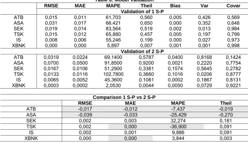
In holdout forecasting, the last few data points are removed from the data series. The remaining historical data series is called in-sample data, and the holdout data is called out-of-sample data. Parameters are optimized by minimizing the fit error measure for in-sample data. After the parameters are optimized, the forecasts for the holdout periods (p periods) are calculated. As portrayed in Table 6, the error statistics (RMSE, MAE, MAPE) are out-of-sample statistics, based on only the numbers in the hold-out period. Other statistics such as Theil's U is an in-sample statistics, based on the non-holdout period. Final forecasting is performed on both the in-sample and out-of-sample periods using the standard technique.
Table 6: Model Validation
RMSE MAE MAPE Theil Bias Var Covar Validation of 1 S-P
ATB 0,015 0,011 61,703 0,560 0,005 0,426 0,569
ASA 0,031 0,017 66,421 0,650 0,000 0,352 0,648
SEK 0,019 0,014 83,564 0,519 0,002 0,013 0,984
TSK 0,015 0,012 65,880 0,457 0,005 0,197 0,799
IS 0,008 0,006 55,246 0,199 0,000 0,027 0,973
XBNK 0,000 0,000 5,897 0,007 0,001 0,001 0,998
Validation of 2 S-P
ATB 0,0319 0,0224 69,1400 0,5787 0,0400 0,8168 0,1424
ASA 0,0700 0,0500 91,8500 0,9200 0,0021 0,2220 0,7754
SEK 0,0167 0,0106 51,2900 0,3381 0,1574 0,5645 0,2782
TSK 0,0133 0,0116 102,7800 0,3660 0,1016 0,0206 0,8777
IS 0,0065 0,0052 45,3600 0,1081 0,0002 0,1867 0,8131
XBNK 0,0003 0,0002 2,0530 0,0044 0,0050 0,0729 0,9221
Comparison 1 S-P vs 2 S-P
RMSE MAE MAPE Theil
ATB -0,017 -0,012 -7,437 -0,019
ASA -0,039 -0,033 -25,429 -0,270
SEK 0,002 0,003 32,274 0,181
TSK 0,002 0,000 -36,900 0,091
IS 0,002 0,001 9,886 0,091
XBNK 0,000 0,000 3,844 0,003
For both Islamic banks the SP1 models have lower errors that SP2 models, whereas for conventional banks SP1 models have higher errors (Table 6).
When SPs are compared, for both GARCH and EGARCH models, SP1 has higher volatility for conventional banks BUT 2 Islamic banks almost predominantly have higher VP in SP2 (there is a clear pattern), thus it makes sense that Islamic bank models work better in SP1, where the AKP government won with a majority vote.
6. CONCLUSION
REFERENCES
Álvarez-Díaz, M., Hammoudeh, S., & Gupta, R. (2014). Detecting predictable non-linear dynamics in Dow Jones Islamic
Market and Dow Jones Industrial Average indices using nonparametric regressions. The North American Journal
of Economics and Finance, 29, 22-35.
Ajmi, A. N., Hammoudeh, S., Nguyen, D. K., & Sarafrazi, S. (2014). How strong are the causal relationships between
Islamic stock markets and conventional financial systems? Evidence from linear and nonlinear tests. Journal of
International Financial Markets, Institutions and Money, 28, 213-227.
Black, F. (1976). The pricing of commodity contracts. Journal of financial economics, 3(1), 167-179.
Clark, P. K. (1973). A subordinated stochastic process model with finite variance for speculative prices. Econometrica:
journal of the Econometric Society, 135-155.
Cox, S. (2002). Retail and private client services. Islamic Finance, Innovation and Growth, Euromoney books and AAOIFI
(London).
Dridi, J., & Hasan, M. (2010). Have Islamic banks been impacted differently than conventional banks during the recent
global crisis. International Monetary Fund. Working Paper, 10, 201.
Ebrahim, M. S., & Safadi, A. (1995). Behavioral norms in the Islamic doctrine of economics: A comment. Journal of
Economic Behavior & Organization, 27(1), 151-157.
El-Gamal, M. A. (2005). Islamic bank corporate governance and regulation: A call for mutualization. Rice University.
Epps, T. W., & Epps, M. L. (1976). The stochastic dependence of security price changes and transaction volumes:
Implications for the mixture-of-distributions hypothesis. Econometrica: Journal of the Econometric Society,
305-321.
Lamoureux, C. G., & Lastrapes, W. D. (1990). Heteroskedasticity in stock return data: volume versus GARCH effects. The
Journal of Finance, 45(1), 221-229.
Fama, E. F. (1965). The behavior of stock-market prices. The journal of Business, 38(1), 34-105.
Gupta, R., Hammoudeh, S., Simo-Kengne, B. D., & Sarafrazi, S. (2014). Can the Sharia-based Islamic stock market returns
be forecasted using large number of predictors and models?. Applied Financial Economics, 24(17), 1147-1157.
Kahneman, D., & Tversky, A. (1979). Prospect theory: An analysis of decision under risk. Econometrica: Journal of the
Econometric Society, 263-291.
Khalichi, A. E., Humayun, K. S., Arouri, M., & Teulon, F. (2014). Are Islamic equity indices more efficient than their conventional counterparts? Evidence from major global index families. Retrieved from http://www.ipag. fr/fr/accueil/la-recherche/publications-WP.
Nelson, D. B. (1991). Conditional heteroskedasticity in asset returns: A new approach. Econometrica: Journal of the
Econometric Society, 347-370.
Mills, P. S., & Presley, J. R. (1999). The Prohibition of Interest in Western Literature (pp. 101-113). Palgrave Macmillan UK.
Willison, B. (2009). Technology trends in Islamic investment banking. Islamic Finance News, 6(19), 22-23.
Yılmaz, D. (2009). Islamic Finance: During and after the global financial crisis. Islamic finance-during and after the global