Proc. IAHS, 371, 59–64, 2015 proc-iahs.net/371/59/2015/ doi:10.5194/piahs-371-59-2015
© Author(s) 2015. CC Attribution 3.0 License.
Open Access
Non-Stationar
ity
and
Extr
apolating
Models
to
Predict
the
Future
(HS02
–
IUGG2015)
Ability of a land surface model to predict climate induced
changes in northern Russian river runoff during the
21st century
O. N. Nasonova1, Y. M. Gusev1, E. M. Volodin2, and E. E. Kovalev1
1Institute of Water Problems, Russian Academy of Sciences, Moscow, Russia 2Institute of Numerical Mathematic, Russian Academy of Sciences, Moscow, Russia
Correspondence to: O. N. Nasonova ([email protected])
Received: 11 March 2015 – Accepted: 11 March 2015 – Published: 12 June 2015
Abstract. The objective of the present study is application of the land surface model SWAP to project cli-mate change impact on northern Russian river runoff up to 2100 using meteorological projections from the atmosphere–ocean global climate model INMCM4.0. The study was performed for the Northern Dvina River and the Kolyma River characterized by different climatic conditions. The ability of both models to reproduce the observed river runoff was investigated. To apply SWAP for hydrological projections, the robustness of the model was evaluated. The river runoff projections up to 2100 were calculated for two greenhouse gas emission scenar-ios: RCP8.5 and RCP4.5 prepared for the phase five of the Coupled Model Intercomparison Project (CMIP5). For each scenario, several runoff projections were obtained using different models (INMCM4.0 and SWAP) and different post-processing techniques for correcting biases in meteorological forcing data. Differences among the runoff projections obtained for the same emission scenario and the same period illustrate uncertainties resulted from application of different models and bias-correcting techniques.
1 Introduction
Nowadays atmosphere–ocean global climate models (AOGCMs) represent the main tool for physically based assessments of future climate change which can be used for hydrological projections. The hydrological projections can be done directly by AOGCMs coupled with river routing models to obtain streamflow at a river basin outlet. This is widely used for evaluating the performance of GCMs and for studying the climate change impact on water resources of large river basins (e.g. Miller and Russell, 1992; Arora and Boer, 2001; Liston et al., 1994). Comparison of runoff hydrographs simulated by GCMs with observed ones (e.g. Arora et al., 2001; Nohara et al., 2006) shows a poor agreement. The major reasons seem to be a coarse spatial scale of GCMs and large errors in modelling precipitation and partitioning precipitation between evapotranspiration and runoff. The alternative approach to direct application of GCMs for runoff projections is application of their outputs to force hydrological models (HMs) or land surface models
(LSMs). For a large river basin or catchment, meteorological outputs can be used directly, while for smaller ones spatial downscaling and disaggregation techniques are used (Arora and Boer, 2001).
In these two approaches a flow routing scheme, as well as HMs and LSMs can also contribute to the accuracy of hy-drograph simulation, however, as it was shown in a number of publications (e.g. Arora et al., 2001; Gosling et al., 2011) this contribution is much smaller as compared to that from a GCM. To reduce biases and uncertainties of any individ-ual GSM, a weighted ensemble mean is suggested to use for multimodel projections (Nohara et al., 2006).
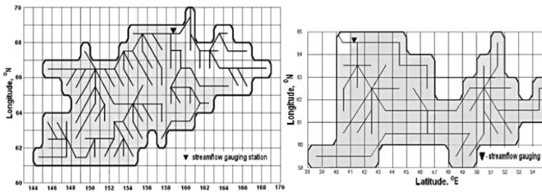
Figure 1.Schematization of the Kolyma (left panel) and the Northern Dvina (right panel) river basins.
uncertainties in river runoff projections resulted from the ap-plication of different types of models (AOGCM and LSM) and different bias-correcting techniques for meteorological projections. Here, AOGCM INMCM4.0 (Institute of Numer-ical Mathematic Climate Model, version 4.0) (Volodin et al., 2010) will be used.
2 Methodology
2.1 Study area
The Northern Dvina and the Kolyma river basins located within the pan-Arctic basin and characterized by different natural conditions were chosen for the study. The North-ern Dvina River basin (area: 357 000 km2) is situated on the north of the European part of Russia. Typical features of the basin are excessive wetness (mean annual precipitation varies from 650 mm in the north to 800 mm in the south-west, while mean annual potential evaporation is within the range of 400–500 mm; 65–70 % of precipitation falls during the warm season), low solar radiation, impact of northern seas, and relatively uniform natural conditions. Air masses from the Atlantic Ocean generally mitigate the climate. The combination of these factors results in a short (3–4 months) and cool summer with mean July temperature equaled to 14– 17◦C and a long (5–6 months) and cold winter with mean January air temperature from−13 to−15◦C. The mean an-nual runoff at the basin outlet is 309 mm. Forests (mostly coniferous) occupy nearly 80 % of the basin.
The Kolyma River basin (area: 644 000 km2) is located in the north-eastern part of Siberia mainly in the subarctic zone, while its northern parts are in the arctic zone. The main fea-tures of this region are extremely low winter temperafea-tures and permafrost. Mean January air temperature varies from
−30 to −42◦C (minimal values reach −50 to −68◦C) in different parts of the basin. Mean July air temperature is 10– 14◦C. Mean annual precipitation increases from 150 mm in the northern part of the basin to 250–300 mm southward and up to 500–600 mm in the mountainous area. Nearly 65–75 %
of precipitation falls during the summer months. The mean annual runoff at the basin outlet is 190 mm. Sparse conifer-ous forests and tundra are prevalent in the basin.
Figure 1 shows schematization of the two river basins using 1◦×1◦ TRIP (Total Runoff Integrating Pathways)
scheme (Oki and Sud, 1998).
2.2 Models
Two models were used for runoff simulation: AOGCM IN-MCM4.0 and LSM SWAP. Both models reproduce runoff at each calculational grid cell. To obtain streamflow at a basin outlet a river routing model (RRM) was used.
2.2.1 INMCM4.0 model
The INMCM4.0 model (Volodin et al., 2010) consists of two major blocks representing a model of general circulation of the atmosphere (with spatial resolution in longitude and lat-itude 2◦×1.5◦) and a model of general circulation of the ocean (1◦×0.5◦).
The INMCM4.0 has participated in a number of interna-tional projects, such as Atmospheric Model Intercomparison Project (AMIP) and Coupled Model Intercomparison Project (CMIP), designed for comparison of GCMs developed by modelling groups in different countries with each other and with observational data. The general conclusion made from the analysis of the obtained results is that the INMCM4.0 by its quality is among the best up-to-date AOGCMs.
2.2.2 SWAP model
reproduces heat and water exchange processes occurring in SVAS.
The last version of SWAP treats the following processes: interception of liquid and solid precipitation by vegetation; evaporation, melting and freezing of intercepted precipita-tion, including refreezing of melt water; formation of snow cover at the forest floor and at the open site; partitioning of non-intercepted precipitation or water yield of snow cover between surface runoff and infiltration into a soil; formation of the water balance of aeration zone including transpiration, soil evaporation, water exchange with underneath layers and dynamics of soil water storage; water table dynamics; for-mation of the heat balance and thermal regime of SVAS; soil freezing and thawing.
2.2.3 River routing model
Runoff modelled by INMCM4.0 or SWAP for each grid box was then transformed by a river routing model. Such a transformation may be performed by different ways. Herein, a simple linear transfer model in river channels was used (Kanae et al., 1995). The RRM operated in a coupled mode with SWAP, and in an offline mode in the case of global model.
2.3 Data
Meteorological outputs and runoff from INMCM4.0’s simu-lations for historical (reference) period (1971–2005) and for two future periods (2026–2045 and 2081–2100), prepared for the phase five of the Coupled Model Intercomparison Project (CMIP5) (Taylor et al., 2012), were used in this study. Pro-jections were performed for two greenhouse gas emission scenarios: a high emissions scenario (RCP8.5) and a medium mitigation scenario (RCP4.5).
Meteorological outputs from INMCM4.0 (precipitation, incoming longwave and shortwave radiation, air temperature and humidity, atmospheric pressure, and wind speed) were used as forcing data to drive the LSM SWAP for runoff sim-ulations. The land surface model parameters for SWAP were prepared using global one-degree datasets provided within the framework of the Global Soil Wetness Project, phase 2 (GSWP-2) (Dirmeyer et al., 2002).
For validation of both models, daily values of streamflow, measured at gauge stations of the rivers (Fig. 1) and kindly provided by Global Runoff Data Centre (GRDC), were used.
2.4 Calibration
2.4.1 SWAP
Since a set of a priori parameters for the SWAP model is based on global datasets, their values identify the basins very approximately and need optimization. Optimization was per-formed automatically against measured daily runoff using the Shuffled Complex Evolution algorithm (SCE-UA) developed
by Duan et al. (1992). The Nash–Sutcliffe coefficient of ef-ficiency NS (Nash and Sutcliffe, 1970) was used as an ob-jective function. The search of the optimum of the obob-jective function was performed under the condition that the absolute value of systematic error|Bias|, calculated as
|Bias| =
P
(xsim−xobs)
P
xobs
·100 % (1)
(wherexsimandxobsare simulated and observed values of a
variablex), does not exceed 5 % (as suggested in Nasonova et al., 2009).
Eight model parameters were calibrated using real meteo-rological forcing data (as in Gusev et al., 2008). Hereinafter, the obtained optimal values of model parameters will be re-ferred to as OPRM-8 (eight optimal parameters under real meteorology).
To reduce possible systematic errors in meteorological variables four correction factors for the most influencing variables (for shortwave and longwave radiation, and sepa-rately for liquid and solid precipitation) were calibrated along with seven model parameters (for details, see Gusev et al., 2008). So, in this case 11 parameters were calibrated. The obtained set of optimal values of model parameters and cor-rection factors will be referred to as OPRM-11.
2.4.2 INMCM4.0
Instantaneous runoff, simulated by INMCM4.0, was trans-formed by a river routing model to obtain streamflow at a river basin outlet. In so doing the effective velocity of wa-ter movement in a channel network was manually optimized using daily river runoff measurements.
2.5 Bias correction in meteorological forcing data
Since meteorological variables simulated by AOGCM IN-MCM4.0 contain systematic errors (biases) several ap-proaches were used to correct variables before using them as inputs for SWAP. First, a correction factor for each me-teorological variable was computed as the ratio of measured variable, averaged over each river basin and over the refer-ence period, to corresponding simulated value. The correc-tion factors were then applied to the AOGCM-simulated 3 h meteorological fields (the corrected fields will be referred to as COR1).
0 1 2 3 4 5
observation simulation
D
ai
ly
r
unoff, m
m
/day
Sample 1
I II III IV V VI VII VIII IX X XI XII
Month
NS=0.88 Bias= -3%
0 1 2 3 4 5
observation
simulation
Sample 2
I II III IV V VI VII VIII IX X XI XII
D
a
ily
r
u
n
o
ff, m
m
/d
a
y
Month
NS=0.88 Bias= 12%
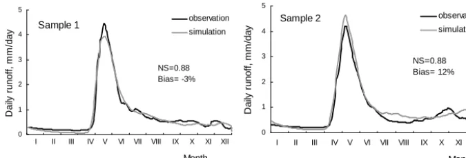
Figure 2.Comparison of measured and simulated by SWAP hydrographs of daily runoff for the Northern Dvina River averaged over the Sample 1 (calibration) and Sample 2 (validation).
account (monthly-3-hourly data were calculated rather than monthly mean values). The corrected 3-hour meteorological fields will be referred to as COR2.
The third approach represents recalibration of SWAP model using meteorological forcing data simulated by AOGCM. The obtained set of optimal values of model pa-rameters and correction factors will be referred to as OPGM-11 (OPGM-11 optimal parameters under GCM’s meteorology). One more recalibration of SWAP was performed for hybridized meteorological data COR2. The obtained optimized parame-ters will be referred to as OPHM-11.
3 Results
3.1 Investigating SWAP model robustness
In order to make sure that model parameter values, obtained for the current conditions, remain valid in projection peri-ods, SWAP model transposability in time under contracted climate conditions was analyzed before its application for hydrological projections. In so doing, model calibration and validation was performed for contrasted climatic conditions in terms of temperature and precipitation. Here, the Northern Dvina River will be considered. We have chosen five years (hereinafter, referred to as Sample 1) with the lowest annual values of precipitation and air temperature during the refer-ence period. The model parameters were optimized for these years (model simulations were performed for the whole ob-servational period). Then the optimized values of model pa-rameters were used for runoff simulation for seven years (re-ferred to as Sample 2) with the highest annual values of pre-cipitation and air temperature. The difference between mean annual values of air temperature in these two samples was nearly 2◦C, while the difference between annual
precipita-tion was about 15 %. Such changes in temperature and pre-cipitation are often projected by the end of XXI century for the pan-Arctic region in different climate change scenarios.
Modeled hydrographs of daily river runoff averaged over the years from the Sample 1 and Sample 2, respectively, are given in Fig. 2. As can bee seen, hydrographs simulated for the Sample 2 using the model parameters optimized for the
Sample 1 are in a good agreement with measured hydro-graphs. The Nash–Sutcliffe coefficients of efficiency are high for both samples. Bias is greater in the Sample 2, neverthe-less, it can be treated as satisfactory.
Thus, it can be concluded that the SWAP model, calibrated for a particular river basin for the driest and coldest years, can be applied with the same optimized parameters in the case of increasing air temperature and precipitation, i.e. the model is rather robust.
3.2 Simulating historical river runoff by SWAP and INMCM4.0 models
Table 1 summarizes statistics characterizing how AOGCM INMCM4.0 and LSM SWAP reproduce river runoff during historical periods. Simulations by SWAP were performed us-ing meteorological outputs from INMCM4.0 with and with-out post-processing bias-correction and with different sets of optimal parameters. As can be seen, recalibration of SWAP’s parameters together with correcting factors for precipitation and radiation provided the best results (see OPGM-11 in Ta-ble 1) for both rivers. As to INMCM4.0, it showed good results for the Northern Dvina River, while for the Kolyma River the performance was poor (and INMCM4.0 will not be used for hydrological projections for the Kolyma River) due to overestimation of simulated precipitation by 90 %.
3.3 River runoff projections and their uncertainties
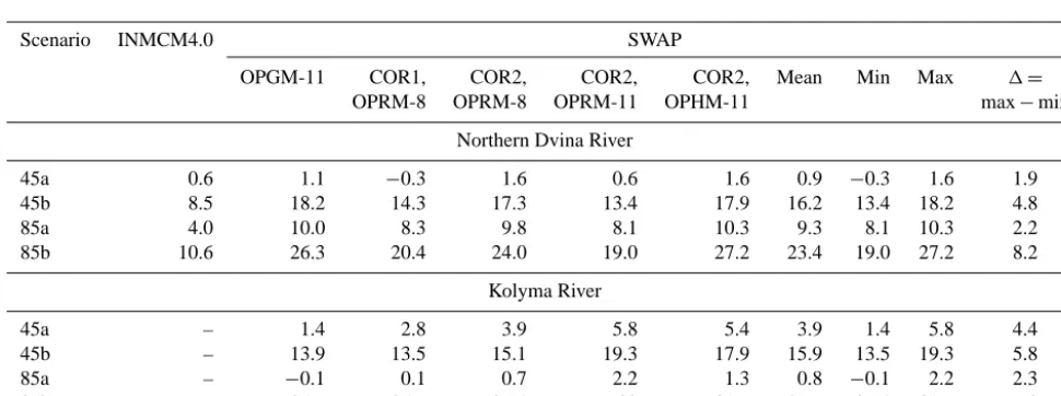
The river runoff projections were obtained for two green-house gas emission scenarios: RCP4.5 and RCP8.5 and for two periods: (a) 2026–2045 and (b) 2081–2100. For conve-nience, they will be referred to as 45a and 45b, and 85a and 85b. Table 2 summarizes projected relative changes of an-nual river runoff (normalized by mean anan-nual runoff during the reference period equaled to 294 mm yr−1for the North-ern Dvina River and to 193 mm yr−1for the Kolyma River) simulated by INMCM4.0 and SWAP.
uncertain-Table 1.Statistical characteristics of river runoff simulations (xsim) performed by the LSM SWAP with different sets of optimal parameters
and different bias-correction techniques and by the AOGCM INMCM4.0 (NS was calculated for monthly values).
Statistics INM-CM4.0 SWAP
OPRM-8 OPGM-11 COR1, COR2, COR2, COR2,
OPRM-8 OPRM-8 OPRM-11 OPHM-11
Northern Dvina River (1972–2003)
xsim, mm yr−1 284 344 294 275 266 272 284
xsim/xobs 0.97 1.17 1.00 0.94 0.90 0.93 0.97
Bias, % −3.8 16.8 0.1 −6.4 −9.9 −7.8 −3.6
NS 0.70 0.60 0.77 0.73 0.63 0.68 0.73
Kolyma River (1978–1998)
xsim, mm yr−1 371 370 200 197 166 165 196
xsim/xobs 1.92 1.92 1.04 1.02 0.86 0.85 1.02
Bias, % 92.0 92.0 3.5 2.2 −14.0 −14.8 1.5
NS −0.20 −0.46 0.64 0.63 0.57 0.57 0.62
Table 2.Relative change in annual runoff (%) of the Northern Dvina and the Kolyma rivers obtained by the LSM SWAP with different sets of optimal parameters and different bias-correction techniques and by the AOGCM INMCM4.0. Mean, maximum and minimum values are given for the SWAP’s projections.
Scenario INMCM4.0 SWAP
OPGM-11 COR1, COR2, COR2, COR2, Mean Min Max 1=
OPRM-8 OPRM-8 OPRM-11 OPHM-11 max−min
Northern Dvina River
45a 0.6 1.1 −0.3 1.6 0.6 1.6 0.9 −0.3 1.6 1.9
45b 8.5 18.2 14.3 17.3 13.4 17.9 16.2 13.4 18.2 4.8
85a 4.0 10.0 8.3 9.8 8.1 10.3 9.3 8.1 10.3 2.2
85b 10.6 26.3 20.4 24.0 19.0 27.2 23.4 19.0 27.2 8.2
Kolyma River
45a – 1.4 2.8 3.9 5.8 5.4 3.9 1.4 5.8 4.4
45b – 13.9 13.5 15.1 19.3 17.9 15.9 13.5 19.3 5.8
85a – −0.1 0.1 0.7 2.2 1.3 0.8 −0.1 2.2 2.3
85b – 25.6 25.7 25.4 30 31.7 27.7 25.4 31.7 6.3
ties resulted from the application of different bias-correction techniques for meteorological forcing data. As can be seen from the Table 2, differences among SWAP’s projections are rather small and do not exceed 8.2 % for both rivers. Differ-ences between projections from two models are larger. Both models project an increase in river runoff for the Northern Dvina River, however, SWAP’s projections are nearly twice larger than corresponding projections form INMCM4.0.
4 Conclusions
The ability of LSM SWAP and AOGCM INMCM4.0 to re-produce runoff of the Northern Dvina and the Kolyma rivers was investigated. AOGCM INMCM4.0 performs fairly well for the Northern Dvina River, while for the Kolyma the
re-sults are very poor. As to SWAP, application of optimal pa-rameter values obtained for real meteorology does not pro-vide a good accuracy of streamflow simulation (especially for the Kolyma River) when meteorological outputs from AOGCM drive the model. Application of bias-correction techniques for AOGCM’s meteorology provides better agree-ment between simulated and measured river runoff.
Due to non-stationary nature of climate the SWAP model robustness was investigated before its application for hydro-logical projections. It was shown that SWAP is quite robust and can be applied for climate change studies.
bias-correction techniques is fairly small (does not exceed 8 %), while differences between changes in runoff projected by two models are larger. On the average, SWAP produces increase in runoff for the Northern Dvina River twice larger than IN-MCM4.0.
Acknowledgements. The study was supported by the Russian Science Foundation (grant No. 14-17-00700).
References
Arora, V., Seglenieks, F., Kouwen, N., and Soulis, E.: Scaling as-pects of river flow routing, Hydrol. Process., 15, 461–477, 2001. Arora, V. K. and Boer, J.: Effects of simulated climate change on the hydrology of major river basins, J. Geophys. Res., 106, 3335– 3348, 2001.
Dirmeyer, P., Gao, X., and Oki, T.: The Second Global Soil Wet-ness Project. Science and Implementation Plan, IGPO Publica-tion Series, InternaPublica-tional GEWEX Project Office, Silver Spring, 37, 1–75, 2002.
Duan, Q., Sorooshian, S., and Gupta, V. K.: Effective and efficient global optimization for conceptual rainfall runoff models, Water Resour. Res., 28, 1015–1031, 1992.
Gosling, S. N., Taylor, R. G., Arnell, N. W., and Todd, M. C.: A comparative analysis of projected impacts of climate change on river runoff from global and catchment-scale hydrological mod-els, Hydrol. Earth Syst. Sci., 15, 279–294, doi:10.5194/hess-15-279-2011, 2011.
Gusev, E. M. and Nasonova, O. N.: Simulation of heat and water exchange at the land–atmosphere interface on a local scale for permafrost territories, Euras. Soil Sci., 37, 1077–1092, 2004. Gusev, E. M. and Nasonova, O. N.: Modelling heat and water
ex-change between the land surface and the atmosphere, Nauka, Moscow, 2010.
Gusev, E. M., Nasonova, O. N., Dzhogan, L. Y., and Kovalev, E. E.: The Application of the land surface model for calculating river runoff in high latitudes, Water Resources, 35, 171–184, 2008.
Gusev, Y. M. and Nasonova, O. N.: Modelling heat and water ex-change in the boreal spruce forest by the land-surface model SWAP, J. Hydrol., 280, 162–191, 2003.
Kanae, S., Nishio, K., Oki, T., and Musiake, K.: Hydrograph esti-mations by flow routing modeling from AGCM output in major basins of the world, Annu. J. Hydraul. Eng., 39, 97–102, 1995. Liston, G. E., Sud, Y. C., and Wood, E. F.: Evaluatig GCM land
sur-face hydrology parameterizations by computing river discharges using a runoff routing model: Application to the Mississippi Basin, J. Appl. Meteorol., 33, 394–405, 1994.
Miller, J. R. and Russell, G. L.: The impact of global warming on river runoff, J. Geophys. Res., 97, 2757–2764, 1992.
Nash, J. E. and Sutcliffe, J. V.: River flow forecasting through con-ceptual models: 1 A discussion of principles, J. Hydrol., 10, 282– 290, 1970.
Nasonova, O. N., Gusev, Y. M., and Kovalev, Y. E.: Investigating the ability of a land surface model to simulate streamflow with the accuracy of hydrological models: A case study using MOPEX materials, J. Hydrometeorol., 10, 1128–1150, 2009.
Nohara D., Kiton, A., Hosaka, M., and Oki, T.: Impact of Climate change on river discharge projected by multimodal ensemble, J. Hydrometeorol., 7, 1076–1089, 2006.
Oki, T. and Sud, Y. C.: Design of Total Runoff Integrating Pathways (TRIP) – A global river channel network, Earth Interact., 2, 1–37, 1998.
Taylor, K. E., Stouffer, R. J., and Meehl, G. A.: An Overview of CMIP5 and the experiment design, B. Am. Meteorol. Soc., 93, 485–498, 2012.
Volodin, E. M., Diansky, N. A., and Gusev, A. V.: Simulating present-day climate with the INMCM4.0 coupled model of the atmospheric and oceanic general circulations, Izvestiya, Atmos. Ocean. Phys., 46, 414–431, 2010.