Proc. IAHS, 372, 437–442, 2015 proc-iahs.net/372/437/2015/ doi:10.5194/piahs-372-437-2015
© Author(s) 2015. CC Attribution 3.0 License.
Open Access
Pre
v
ention
and
mitigation
of
natur
al
and
anthropogenic
hazards
due
to
land
subsidence
3-D land subsidence simulation using the NDIS package
for MODFLOW
D. H. Kang and J. Li
Department of Civil Engineering, Morgan State University, Baltimore, Maryland, USA
Correspondence to: J. Li ([email protected])
Published: 12 November 2015
Abstract. The standard subsidence package for MODFLOW, MODFLOW-SUB simulates aquifer-system
com-paction and subsidence assuming that only 1-D-vertical displacement of the aquifer system occurs in response to applied stresses such as drawdowns accompanying groundwater extraction. In the present paper, 3-D movement of an aquifer system in responses to one or more pumping wells is considered using the new aquifer-system deformation package for MODFLOW, NDIS. The simulation of aquifer- system 3-D movement using NDIS was conducted with a stress or hydraulic head dependent specific storage coefficient to simulate nonlinear defor-mation behavior of aquifer-system sedimentary materials. NDIS’s numerical simulation for aquifer horizontal movement is consistent with an analytic solution for horizontal motion in response to pumping from a leaky confined aquifer (Li, 2007). For purposes of comparison, vertical subsidence of the aquifer system in response to groundwater pumping is simulated by the both the NDIS and MODFLOW-SUB models. The results of the simulations show that land subsidence simulated by MODFLOW-SUB is significantly larger and less sensitive to pumping rate and time than that simulated by NDIS. The NDIS simulations also suggest that if the total pumpage is the same, pumping from a single well may induce more land subsidence than pumping from multiple wells.
1 Introduction
Land subsidence has been attributed to the compaction (com-pression) of aquifer systems caused by ground-water with-drawal. Widespread land subsidence caused by the overex-ploitation of groundwater is a global problem. Over the past decades, many experts have attempted to develop models to evaluate transient aquifer-system compaction and subsi-dence accurately and efficiently using MODFLOW (Leake and Prudic, 1991; Hoffmann et al., 2003; Leake and Gal-loway, 2007). Most of the developed models only account for the 1-D-vertical displacement that is known to be associ-ated with changes in aquifer-system storage, attributed prin-cipally to aquitards-fine-grained, low permeability interbeds and confining units. However, the occurrence of horizontal movement caused by ground water withdrawal indicates that aquifer-system deformation and subsidence result from 3-D movement of the aquifer system. The NDIS numerical model presented here simulates 3-D displacement of the solid ma-trix caused by groundwater extraction, and is based on the
principle of effective stress for the case of a constant geo-static load.
The purpose of this paper is to present the NDIS numeri-cal model for 3-D aquifer-system movement due to ground-water withdrawal, and to evaluate NDIS with respect to the simulated aquifer- system vertical movement (subsidence) by comparing simulation results from NDIS with those from MODFLOW-SUB. One of the advantages of the approach presented in this paper is that one can simplify the processes of solving for 3-D aquifer-system deformation with stress-dependent aquifer-system specific storage coefficients that change due to compaction driven by hydraulic force loading on the aquifer-system skeleton.
2 Theoretical background for the NDIS model
2.1 Basic equation
∇ ·(K∇h)+W=Ss
∂h
∂t, (1)
where h is hydraulic head; K is hydraulic conductivity, a
diagonal matrix of rank two; W denotes a volumetric flux
per unit volume and represents sources and/or sinks of wa-ter mass within an aquifer system; andSs(=Ssk+Ssw) is the
specific storage coefficient, where Ssk andSsware the
spe-cific storage coefficients of the soil skeleton and pore water, respectively, andSskcan be either a constant for linear elastic
materials or a stress-dependent variable for inelastic materi-als. The individual solid particles are assumed to be incom-pressible. The termWdenotes a volumetric flux per unit vol-ume and represents sources and/or sinks of water mass within an aquifer system. For an aquifer system that has steady flow without the termW, Eq. (1) can be further simplified to the Laplace equation. The US Geological Survey (USGS) devel-oped the 3-D program MODFLOW that numerically simu-lates steady and transient groundwater flow. To simulate land subsidence in response to groundwater withdrawal, USGS further developed the MODFLOW-SUB package simulating 1-D aquifer-system compaction and subsidence based on ver-tical stress and strain of the aquifer system. In contrast, a new 3-D model, NDIS developed from DIS (Zhang, 2009) sim-ilarly uses the parent program MODFLOW-96 (McDonald and Harbaugh, 1988) and the bulk flux relation through per-meable, deformable and saturated porous materials. The bulk flux relation is defined by Helm (1979, 1984):
qb(x, y, z, t)=vs(x, y, z, t)+q(x, y, z, t), (2)
where qb is the bulk flux; vs is the velocity of solids; q
is the transient specific discharge that is defined by q=
n(vs−vw); andvw is the fluid (water) velocity. Note that a
bolded variable with an arrow represents a vector throughout this paper.
For steady flow, Eq. (2) can be expressed by the following form:
qb−st(x, y, z)=vs−st(x, y, z)+qst(x, y, z), (3)
where the subscripts st denote the steady flow. If no aquifer movement is assumed once an equilibrium condition (or steady flow) is reached, i.e., vs−st(x, y, z)=0, and the
bulk flux is assumed to be constant, i.e., qb(x, y, z, t)= qb−st(x, y, z), combining Eqs. (2) and (3) results in:
vs(x, y, z, t)= −[q(x, y, z, t)−qst(x, y, z)]. (4)
The expression (4) indicates that aquifer velocity can be written in terms of the specific discharge for transient and steady flow. Moreover, on the right side of Eq. (4), the terms q(x, y, z, t) andqst(x, y, z) can be found by running MOD-FLOW for transient flow and steady flow, respectively. It should be pointed out that the assumption ofvs−st(x, y, z)=
0 suggests that deformation due to secondary consolidation is negligible and the assumption of the constant bulk flux im-plies a constant pumping rate. The former means that the aquifer system has no further displacement or deformation once the unsteady flow becomes steady one that is under the equilibrium condition, and the latter can be proved to be true for a constant pumpage (Li and Helm, 2010). Therefore, the velocity field of solidsvsfor transient flow can be computed
as a function of space and time from Eq. (4). Using Eq. (4), the displacement field of solids,uscan be further computed
through integrating the velocity field of solids over the time as follows:
us=
t Z
t0
vsdt+us0, (5)
where subscript 0 stands for the initial value of displacement and time. The velocity and displacement fields of the solid skeleton vary with time.
2.2 Stress-dependent specific storage coefficient
Based on an exponential relation between the effective vol-ume stress and volvol-ume strain of the soil skeleton, the specific storage coefficient can be found to be a function of volume stress written in the following form (Li and Ding, 2013):
Ssk(σv0),αγw=Ssk0
σv00
σ0
v
, (6)
whereαis the compressibility of the soil skeleton;Ssk0(=
γwα0) is the initial specific storage coefficient, where the
symbol , stands for “by definition”,γw is the water unit
weight and α0 is the initial compressibility of the aquifer
system;σv00 is the initial effective volume stress;σv0 is the current effective volume stress and the subscript 0 denotes the initial value of a variable throughout this paper. Because the effective volume stress is equal or larger than its ini-tial value (Ssk≤Ssk0att≥0), suggests that in response to
changes in hydraulic head due to groundwater extraction, an aquifer system with elastic materials may deform larger than that with inelastic materials because of the strain-hardening effect. Equation (6) can be written in terms of transient
hy-draulic head,h through Terzaghi’s principle (1925) of
ef-fective stress: σv=σv0+p and Hubbert’s potential (1940):
h=z+p/γw in terms of hydraulic head in the following
form:
Ssk(h)=Ssk0
σv00
σv−γw(h−z)
, (7)
whereσvis the total volume stress and is normally assumed
to be constant;zdenotes the elevation from a chosen datum; pis the pore water pressure.
Note thatSsk(h) in Eq. (7) can be used in Eq. (1) because
D. H. Kang and J. Li: 3-D land subsidence simulation using the NDIS package for MODFLOW 439
nonlinear partial differential equation (PED) for hydraulic head. For simplicity, the constantSske0is applied to Eq. (1)
for elasticity when σv0≤σv0−pre and the head-dependent
Sskv(h)=Sskv0σv00 /σ
0
v for inelasticity whenσv0>σv0−prethat
is preconsolidation stress.
3 Numerical modeling
The finite-difference numerical simulation is based on a con-ceptual model that consists of five thin aquitards (thickness is 1 m for each) and two aquifers (thickness is 30 m for each). The top layer (Layer 1) is an unconfined aquifer and the bot-tom layer (Layer 7) is a confined aquifer. Layers 2–6 are aquitards that serve as a hydraulic separator between two aquifers. The schematic of the seven layer aquifer system is
shown in Fig. 1 in which Qis the pumping rate, andH is
the total thickness (65 m) of the aquifer system. The option of “no delay” in MODFLOW-SUB is chosen for simulation of the aquifer-aquitard system.
The lateral boundaries of the conceptual model are speci-fied as constant-head boundaries. The initial head is assumed to be zero. Summary properties of the aquifer system are given in Table 1.
To simulate 3-D land movement at a basin-wide scale in an efficient and accurate way, the seven-layer aquifer system is discretized horizontally, and each layer is represented by a grid of 37 rows by 37 columns. The total number of elements (model cells) equals 9583.
Two cases are simulated for purposes of comparison. For one case, a single well is simulated at row 19 and column 19 in the confined aquifer in Layer 7, and for the second case of three pumping wells are also simulated. In the three-well case, the centre well is located at the same location as for the one-well case, and the other two wells are located on a line passing through the centre well. As indicated in Eq. (7), Sskv requires specification of the four parametersSskv0,σv,
σv00 andz, respectively. The parameterSskv0 is given in
Ta-ble 1 and the values of the other three parameters in each layer are calculated and shown in Fig. 1, where the stress parameters are evaluated using the weight of the overbur-den material (geostatic load) and the initial head (h0) where
σv00 =σv−γw(h0−z). The soil unit weight is 21.0 kN m−3
for the aquifer material and 18.5 kN m−3 for the aquitard material. The empirical formulae are introduced to findK0,
the coefficient of earth pressure at rest, so that the volume stress can be evaluated from the vertical stress. In this pa-per,K0=0.19+0.233 log(PI) for clay andK0=1−sinϕfor
sand are used, respectively, where PI and ϕ are the plastic index and the internal friction angle, respectively. The to-tal volume stress can be further calculated using the rela-tionσv=σz(1+2K0)/3. For simplicity, the preconsolidation
head is not introduced to each model layer although NDIS is capable to compute both elastic and inelastic deformation.
Page 13
H =65.0m
Q
Unconfined Aquifer (30m)
Well
Confined Aquifer (30m)
4
Layer 𝛔𝐯 𝛔𝐯𝐯′ Z(m)
1 315.00 165.00 -15.0 2 564.25 334.25 -30.5 3 582.75 342.75 -31.5 4 601.25 351.25 -32.5 5 619.75 359.75 -33.5 6 638.25 368.25 -34.5 7 1050.00 537.50 -50
5
17 18 19 20 21
Drawdown Curve
Piezometric Surface
Aquitard
Impermeable
Figure 1.A conceptual model of an aquifer-aquitard system and
the values ofσvandσv00 at different depths.
Table 1.Properties of the conceptual model.
Layer
Properties 1 2 to 6 7
Kh(m d−1)∗ 1.00×101 1.00×10⁻² 1.00×101
Kv(m d−1)∗ 1.00 1.00×10⁻³ 1.00
Sskv0 1.00×10⁻⁴ 1.00×10⁻² 5.00×10⁻³
Sske0 1.00×10⁻⁵ 1.00×10⁻³ 5.00×10⁻⁴
Thickness (m) 3.00×101 1.00 3.00×101
Layer σv(kPa) σv00 (kPa) Z(m)
1 315.00 165.00 −15.0
2 564.25 334.25 −30.5
3 582.75 342.75 −31.5
4 601.25 351.25 −32.5
5 619.75 359.75 −33.5
6 638.25 368.25 −34.5
7 1050.00 537.50 −50
∗K
h,Kv– horizontal and vertical hydraulic conductivities, respectively.
Four criteria specified in the numerical solver (Strongly Implicit Procedure package) in MODFLOW are: (1) the error criterion=0.0001; (2) the acceleration parameter=1.0; (3)
the maximum number of iterations=500; (4) seed=0.001
(specified for calculation of iteration parameter). The com-putation starts by running MODLFOW for steady flow and then proceeds for transient flow with MODFLOW again ac-cording to Eq. (4).
Three different values of hydraulic diffusivity of the con-fining layer,cv=K/Ss(1000, 2000, and 4000 m2day−1) are
0 0.05 0.1 0.15 0.2 0.25
0 900 1800 2700 3600
L a nd Su bs idence (m )
Distance from the center well (m)
NDIS MODFLOW-SUB 0 0.05 0.1 0.15 0.2 0.25
0 900 1800 2700 3600
L a nd Su bs idence( m )
Distance from the center well (m)
MODFLOW-SUB NDIS
A) B)
Figure 2.Comparison of land subsidence predicted by the NDIS
and MODFLOW-SUB after 100 days pumping; (a) Land subsi-dence for a single well, (b) Land subsisubsi-dence for three wells after 100 days pumping.
-0.8 -0.6 -0.4 -0.2 0
0 600 1200 1800 2400 3000 3600
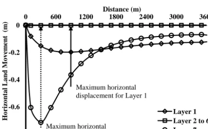
H o rizo nta l L a nd M o v em ent (m ) Distance (m) Layer 1 Layer 2 to 6 Layer 7 Maximum horizontal
displacement for Layer 1
Maximum horizontal displacement for Layer 7
Figure 3.Horizontal subsidence after 100 day pumping simulated
by NDIS.
4 Resulsts and analysis
Subsidence (cumulative model layer compaction) simulated by NDIS and MODFLOW-SUB is shown in Fig. 2a and b.
A pumping rate of 1000 m3day−1 and a pumping period
100 days for both the single-well and three-well are simu-lated to evaluate the displacements. In the three-well case, the center well is located at the same location as for the one-well case, and the other two one-wells are located on each side of the center well along a line passing through it. The results show that the maximum subsidence for both models occurs near the well. Subsidence decreases rapidly with distance from the pumping well similar to the nature of the draw-down. The results indicate that the subsidence simulated by MODFLOW-SUB is significantly larger than that simulated by NDIS (Fig. 2). It is interesting to note that even though the total pumping rate in both the one-well and three-well cases are the same (i.e., 1000 m3day−1), land subsidence in response to three pumping wells is much less than that due to a single well. However, for the three-well case at the location between two pumping wells subsidence simulated by NDIS is slightly larger than that by MODFLOW-SUB (Fig. 2b).
u = 0.0479ln(t) - 0.0259 R² = 0.9917
u = 0.0082ln(t) - 0.0154 R² = 1
0 0.05 0.1 0.15 0.2 0.25 0.3 0.35
0 200 400 600 800 1000
L a nd Su bs idence (m )
Pumping Time t (day)
MODFLOW-SUB
NDIS
u = 0.0002Q- 0.0008 R² = 1
u = 2E-05Q + 0.0004 R² = 1
0 0.5 1 1.5 2 2.5
0 2000 4000 6000 8000 10000
L a nd Su bs idence (m )
Pumping Rate Q (m3/day)
MODFLOW-SUB
NDIS
A) B)
Figure 4.Sensitivity comparison using NDIS and
MODFFLOW-SUB models. (a) Land subsidence vs. pumping rate. (b) Land sub-sidence vs. pumping time.
For horizontal movement (Figs. 3 and 5), the numerical so-lutions for the aquifer system with a leaky confining unit are consistent with the analytic solution developed by Li (2007). Namely, the aquifer movement has two zones. One is a com-pression zone and the other is an extension zone. The posi-tion of the boundary between the two zones is a funcposi-tion of time. This is because in the vicinity of the pumping well, the displacement of the solid matrix approaches zero as the well screen is assumed to be permeable only to water. The inward moving grains tend to accumulate in the surrounding area of the well and form a compression zone around the well that extends outward from the well as pumping continues.
The aquifers (Layers 1 and 7) show significant horizon-tal movement compared with the aquitards where there is negligible horizontal motion. Large radial strain occurs un-der compression near the well and decreases to zero at a transient point of the maximum radial displacement (Fig. 3). Similar to the relation between vertical displacement and dis-tance from the pumping well, for horizontal displacement be-yond the point of maximum horizontal motion the horizontal displacement gradually decreases along the radial direction. The displacement curves for all layers eventually approach the constant head boundary where strain becomes zero. The peak horizontal displacements in the confined (Layer 7) and unconfined aquifer (Layer 1) occur at about 300 and 700 m from the pumping well, respectively (Fig. 3).
Sensitivity analyses were conducted for different pumping rates and discharge periods to evaluate movement sensitivity using the NDIS and MODFLOW-SUB models. The results show that increasing pumping rate and time cause increases in displacements. Figure 4a and b show that subsidence sim-ulated by NDIS is less sensitive than that by MODFLOW-SUB to changes in the pumping rate and time.
con-D. H. Kang and J. Li: 3-D land subsidence simulation using the NDIS package for MODFLOW 441
-0.001 0 0.001 0.002 0.003 0.004
0 0.1 0.2 0.3 0.4 0.5 0.6
0 600 1200 1800 2400 3000 3600
St
ra
in
H
or
iz
on
tal
M
ove
m
en
t (
m
)
Distance from Well (m)
Horizontal strain Horizontal displacement The max displacement at (300, 0.5)
Compression Extension
Figure 5.Horizontal movement and strain in Layer 7 after 100 days
pumping.
0
0.01
0.02
0.03
0.04
0.05
0 900 1800 2700 3600
L
a
nd
Su
bs
idence
(m
)
Distance from the well (m)
K/Ss =1000
K/Ss = 2000
K/Ss = 4000 -0.8 -0.7 -0.6 -0.5 -0.4 -0.3 -0.2 -0.1 0
0 900 1800 2700 3600
H
o
rizo
nta
l
M
o
v
em
ent
(m
)
Distance from the well (m)
K/Ss = 1000
K/Ss = 2000
K/Ss = 4000
A) B)
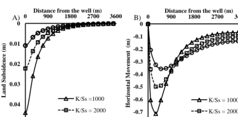
Figure 6. Sensitivity of displacement to hydraulic diffusivity
(m2/day) using the NDIS model (a) Subsidence, (b) Horizontal
movement (Layer 7) after 100 days pumping.
fined aquifer (Layer 7). The peak value of the horizontal land subsidence in Layer 7 is located 300 m from the center of the well. This location is also a transition point between exten-sional and compresexten-sional strain.
Figure 6 shows the impact of hydraulic diffusivity on the vertical and horizontal movement (Layer 7) using the NDIS model. It is interesting to note that the vertical displacement at any location is decreasing along with increasing hydraulic diffusivity. However, this is true for horizontal displacement only when horizontal distance is less than 1000 m. When the horizontal distance larger than 1000 m, the horizontal dis-placement is increasing with increasing hydraulic diffusivity. The plots in Fig. 7 compare the sensitivity of verti-cal displacement to hydraulic diffusivity for the NDIS and MODLFOW-SUB models. In general, subsidence decreases with increasing hydraulic diffusivity for the both models. However, the results show subsidence simulated by NDIS is less sensitive to hydraulics diffusivity than that simulated by MODFLOW-SUB.
u = -0.159ln(cv) + 1.4349
R² = 0.9843
u = -0.024ln(cv) + 0.208
R² = 0.9673
0 0.1 0.2 0.3 0.4
0 1000 2000 3000 4000 5000
La
nd Subs
ide
nc
e
(m
)
Diffusivity cv (K/Ss, m2/day)
MODFLOW-SUB NDIS
Figure 7.Comparison between NDIS and MODFLOW-SUB
mod-els for subsidence sensitivity to hydraulic diffusivity,cvis
diffusiv-ity (=K/Ss, m2day−1).
5 Summary and conclusions
The summary and conclusions of this paper are given below:
– A new NDIS module for 3-D aquifer movement has been applied. The NDIS model is incorporated to the parent program MODFLOW-96 that was modified to solve a nonlinear partial differential equation for hy-draulic head.
– Subsidence based on a hypothetical conceptual model is simulated using both the NDIS and MODFLOW-SUB models for purposes of comparison. The results indi-cate land subsidence simulated by MODFLOW-SUB is significantly larger than that simulated by NDIS.
– Two cases are considered for the conceptual model, one case has a single pumping well and the other case has three pumping wells, with two of the wells on opposite ends of a line intersecting, and at equal distances from, a center pumping well. The two cases are simulated with both the NDIS and MODLFOW-SUB models. The re-sults show that for the same total discharge rate, the maximum land subsidence in response to a single pump-ing well is larger than that from the three pumppump-ing wells distributed as described above.
model layers representing the pumped and non-pumped aquifers and are a function of time.
– Sensitivity analysis using NDIS indicates that vertical displacement at a location reduces with increasing dif-fusivity at any location but this is true for horizontal displacement only within a 1000 m radius. Farther than 1000 m from the pumping well, the horizontal displace-ment increases with increasing hydraulic diffusivity.
– Comparison of sensitivity analysis between the NDIS and MODLFOW-SUB models shows vertical move-ment decreases with increasing of pumping rates and time for both the models. However, land subsidence simulated by NDIS is less sensitive to both the pumping rate and time than that simulated by MODFLOW-SUB.
Acknowledgements. The research and writing of this paper were
supported by US Department of Energy under the contract DE-NA0000720 through the Samuel P. Massie Chairs of Excellence Program.
References
Bear, J.: Dynamics of fluids in porous media, Dover Publications, Inc., NY, 800 pp., 1972.
Helm, D. C.: A postulated relation between granular subsidence and Darcy’s law for transient flow, in: Evaluation and Prediction of Subsidence, edited by: Saxena, S. K., ASCE, NY, 417–440, 1979. Helm, D. C.: Analysis of sedimentary skeletal deformation in a con-fined aquifer and the resulting drawdown, in: Groundwater Hy-draulic, edited by: Rosenshein, J. S. and Bennett, G. D., Ameri-can Geophysical Union, Washington DC, 29–82, 1984. Hubbert, K. M.: The theory of groundwater motion, J. Geology, 48,
745–944, 1940.
Hoffmann, J., Leake, S. A., Galloway, D. L., and Wilson, A. M.: MODFLOW-2000 ground-water model–user guide to the sub-sidence and aquifer-system compaction (SUB) package, USGS Open-File Report 03–233 Tucson, Arizona, 44 pp., 2003. Leake, S. A. and Galloway, D. L.: MODFLOW ground-water
model–user guide to the subsidence and aquifer-system com-paction package (SUB-WT) for water-table aquifers, US Geo-logical Survey, Techniques and Methods, 6–A23, Reston, VA, 42 pp., 2007.
Leake, S. A. and Prudic, D. E.: Documentation of a computer pro-gram to simulate aquifer-system compaction using the modu-lar finite-difference ground-water flow model: US Geological Survey Techniques of Water- Resources Investigations, Book 6 Modeling Techniques, Chapter A2, US Geological Survey Open-File Report, Reston, VA, 88–482, 1991.
Li, J.: Transient radial subsidence of a confined leaky aquifer due to variable well flow rate, J. Hydrology, 333, 542–553, 2007. Li, J. and Ding, D.: Modeling 3D land subsidence due to
ground-water pumping with a variable parameter, Global View of En-gineering Geology and the Environment, Beijing, China, CRC Press, Taylor & Francis Group, New York, 457–462, 2013. Li, J. and Helm, D. C.: A theory of three-dimensional land motion
in terms of its velocity field, Land Subsidence, the Proceedings of the 8th International Symposium on Land Subsidence, 17– 22 October 2010, Queretaro, Mexico, 475–483, 2010.
McDonald, M. G. and Harbaugh, A. W.: A modular three-dimensional finite-difference ground-water flow model, Tech-niques of Water-Resources Investigations of the USGS: Chapter A1, Book 6, USGS, USGS, Reston, VA, 586 pp., 1988. Terzaghi, K.: Settlement and consolidation of clay, Eng. News,
Rec., 95, 874–878, 1925.