COMPUTATIONAL TOOL FOR SIMULATION OF THE DYNAMIC
RESPONSE OF VALVE TRAIN
Krešimir Osman1
1 Faculty of Mechanical Engineering and Naval Architecture, University of Zagreb, Croatia
Received 28 March 2013; accepted 4 December 2013
Abstract: This paper presents the development of the MOTORI 2004 computing tool that calculates the distance, speed and acceleration of a car engine valve train’s oscillating mass m, which is reduced to the valve axis. Distance diagrams, speed and accelerations are provided in dependence on the camshaft twist angle at a constant rotational speed in several consecutive revolutions. The computing tool implements a mathematical description and numerical solution for the motion of mass m of a valve gear dynamic model. Valve lift h is given numerically using a series of equidistant points in the period of one camshaft revolution. The variabilities of camshaft rotation and spring thread vibration as a result of cam lift harmonic excitation. The computing solutions were tested at valve opening points and in imaginary extreme operating conditions (soft/hard spring, low/high damping, low/high rotational speed and increased clearance.
Keywords: computational tool, MOTORI 2004, simulation, dynamic response, valve train.
1 Corresponding author: [email protected]
1. Introduction
The importance of engineering information is underlined by the fact that product lifecycle as chain of information transformation processes both dissipates and creates large amounts of information (McAlpine et al., 2006). One way in presenting engineering information can be by applying various computer supported visualizations. It assumes a number of techniques utilized to provide processing, comprehension, and retention of information in static, animated, dynamic, and interactive graphics (Plötzner and Lowe, 2004). Graphical user interfaces with underlying algorithms, through which information can be visualized as spatially organized and interactive, alleviate the information understanding and retrieval
process, thus supporting problem solving that engineer’s face today. Engineering automotive systems is a complex task. Therefore, models and computer simulations are needed to test functions and behaviors of non-existing systems, reduce testing time and cost, reduce the risk involved and detect problems early, which reduces the amount of implementation errors. The visualization is hereby called to display the dynamic relationship between emerging information as input by many sources during dynamic response simulation. Simulation has a major impact on the ability to produce better products.
computing tool is based on the given valve train dynamic model, explained in greater detail in Chapter 3 of this paper. The proposed model is simple enough to obtain satisfactory results without any special measuring equipment, yet complex enough to enable simulating extreme valve train operating conditions and testing the mathematical description. The proposed model’s mathematical description was made according to the method presented by Levy and Wilkinson (1976), which is described in greater detail in Chapter 4 of this paper. The analysis in the paper was performed by defining a camshaft reference model, which is actually a Kurz’s shock-free cam (Kurz, 1954). The paper also defines two imaginary engines with substantially different valve train properties due to (Mahalec, 1996): Motor-1, with a highly stiff valve train, and Motor-2, a representative of cam-in-block engines with long valve lifter rods and rocker arms i.e. low valve train stiffness.
After this chapter, Chapter 2 provides an overview of the research area. Chapter 3 defines a valve train dynamic model, whiles Chapter 4 provides a mathematical description of the model. This is followed by a description of the MOTORI 2004 computing tool in Chapter 5 and a presentation of model testing including and a discussion of the results in Chapter 6 of this paper. The paper ends with a conclusion and a proposal for future research in Chapter 7.
2. State of the Art
The research area overview will first specify the papers that had a significant impact on development of methods and methodologies for mathematical modelling and simulation of camshaft cam profile’s dynamic behaviour followed by an overview of some more recent papers in this area.
Derndinger (1959) in his dissertation was the first to demonstrate a relatively simple method for determining the maximum rotational speed of a valve train. His paper was based on measurements made on car engines at the Mercedes Benz factory in Stuttgart. He based his method on an analytically defined Kurz cam (Kurz, 1954) used in the German automotive industry at the time. It enabled analytical solving of the valve train model motion differential equation, with some simplification of borderline conditions. The method was derived assuming high arbitrary valve spring stiffness, so that the valve cannot be separated from the cam, after which he calculated the first acceleration amplitude on the top of the cam. He compared the inertia force at this point with the force at the highest valve lift. According to the author, an engine can work with a rotational speed higher than the speed so determined because the valve is able to sustain minor jumps. The actual magnitude of this needs to be determined by carrying out experiments for each case. According to the author (Derndinger, 1959), the engine tolerated a speed load of 15% well. His calculation results were quite consistent with the measurement results, so his method has also been published in Levy and Wilkinson (1976).
Wagstaff (1967) was the first who was use a 10-mass model to describe the valve train, 6 of which represented valve spring threads, 2 represented the lifter rod, and one represented each of the valve and lifter shell. He demonstrated that the calculation and measurement error was not so large assuming the vibrations are stationary at the observed rotational speed, because the vibration becomes stable after only 5 to 6 revolutions, depending of the level of damping. The differences between the first cycle and the stable ones were not large.
Hafner (1973) presented a new approach to the valve train vibration problem. He used the solid vibration theory with continuous distribution of mass, stiffness and damping. The most significant value of the paper is in its excellent description of a system with infinite degrees of freedom, which is suitable for the studying of valve spring thread vibration. The paper also indicates that measurements are necessary to determine the exact values of damping constants.
Through mathematical modelling and simulation, experimental validation of results and robust optimal design strategies David et al. (1997), showed in his paper that it was possible to develop optimal design of valve train systems.
Choi et al. (2000) was interested in the elaboration of camshaft lobe profiles using implicit filtering algorithm helping parameter identification and optimization in automotive valve train design.
Cardona et al. (2002) presented a design methodology to design cams for motor engine valve trains using a constrained optimization algorithm in order to maximize
the time integral of the valve area open to gas flow. He observed that profile errors can have a major impact on the dynamic performance of such high-speed follower cam systems.
Kim et al. (1991) used a lumped mass-spring-damper to predict the dynamic behaviour of a cam-valve system that gives concordant results compared with experimental tests for the evaluation of contact forces in the system.
Jeon et al. (1989) stated in his paper that with experimental and simulation results that optimize a cam profile, he is able to increase the valve lift area, while reducing the cam acceleration and the peak pushrod force. The jump phenomenon of the follower observed at certain can also be avoided.
Teodorescu et al. (2012) presented an analysis of a line of valve trains in a four-cylinder, four-stroke in-line diesel engine in order to predict the vibration signature taking into account frictional and contact forces.
Carlini et al. (2002) conducted a series of experimental measurements of valve motion of a motorbike engine and identified the effect of backlash in cam kinematic pairs and the ensuing jump phenomenon.
De Wilde (1967) concluded that it was then necessary to reduce the coefficient of friction by adopting a proper material combination in wear affecting valves.
Dujmović et al. (2005) in their paper presented the dynamic behavior of a single OHC valve train with his parametric mechanical model and numerical solution for different camshaft speeds covering the operational range of the engine.
3. Defining a Valve Train Dynamic Model
Simulation tests showed that incorrect values of the damping constant provide
senseless results even with quite simple models. While complex models with more degrees of freedom enable more detailed analyses of dynamic response, they contain a relatively large number of damping and stiffness constants and this number rapidly increases the risk of obtaining incorrect results. To be able to successfully control such model, a number of experiments need to be carried out and using first-class expensive measuring equipment is inevitable.
2 4
3
1
δ2
lu
h4 = lu - lmin
lmin
+ h
δ3
hBV - z z
m
k3 c3
i3 = + 1
i4 = - 1 i2 = - 1
i1 = + 1
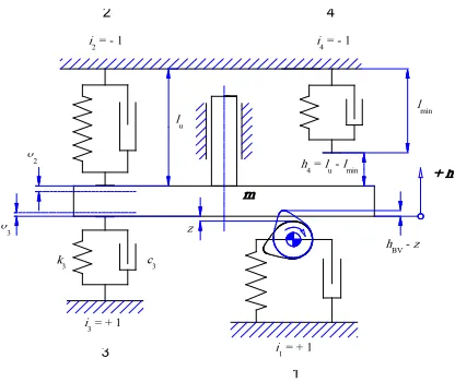
Fig. 1.
Valve Train Dynamic Model Source: Levy and Wilkinson (1976)
Symbols (on Fig. 1): 1 – camshaft and its bedding in the cylinder head, 2 – valve spring and valve guide, 3 – valve seat, 4 – addition increase in valve spring stiffness and damping when the threads interlock; c [kg/s] – damping constant; δ2 [m] – initial (built-in) valve
spring deflection; δ3 [m] – initial valve seat deflection; h [m] – valve lift; hBV [m] – cam
profile lift; h4 [m] – valve lift before the spring threads interlock; i – vibration element
transmission ratio; k [N/m] – stiffness constant; lmin [m] – length of the fully pressed spring,
lu [m] – length of the spring in the built-in condition; m [kg] – oscillating mass reduced to
the valve axis; z [m] – clearance.
On the other hand, the used model having a single degree of freedom, but very refined characteristics, may be kept under control relatively easily. In addition, it represents the valve train in modern engines and race
cars very well and enables very good analysis of valve motion.
• a single degree of freedom,
• four vibration elements in the form of stoppers (they are only able to transmit compressive forces, not tensile) that simulate:
1. the valve train (the camshaft and its bedding in the cylinder head), 2. the valve spring and friction in the
valve guide,
3. the valve seat and the head around the seat,
4. the valve spring when its threads interlock,
• the clearance between the cam and the valve,
• the defined conditions for valve’s seating in the seat and separation from the cam, • all magnitudes are reduced to the valve
axis.
4. Mathematical Description of the Model
The mathematical description contemplates transitional and stationary vibrations. However, the analyses performed by Wagstaff (1967) show that the transitional component shows fatigue after only five to six camshaft revolutions, and this is only detectable if the vibration model incorporates valve spring thread vibration caused by cam lift harmonics. The model used did not take spring thread vibration into account. Namely, the valve spring has by far the lowest damping of all vibration elements of the model. A calculation of spring point shifts in case of free vibrations shows that amplitudes drop very quickly even here.
The mathematical description of the vibration model was made according to the method presented by Levy and Wilkinson (1976).
Balance of forces on mass m:
Resultant F of forces Fj for all vibration
elements acting on mass m is (Eq. (1)):
(1)
where is: i – is the vibration element transmission ratio, j – is the vibration element serial number, and n – is the vibration element total number.
The following rules are applied:
1. the force on the vibration element (spring + damper) is positive if it
compresses the element.
2. considering the obser ved mass, transmission ratio i of the vibration element force is:
• positive - if a positive shift of the observed mass (while the rest are stationary) stretches the element,
• negative - if a positive shift of the observed mass compresses the element.
Forces in vibration elements:
The vibration elements are stopper-shaped, which means they are only able to transmit compressive forces. Their indices are: 1 – camshaft and its bedding in the cylinder head, 2 – valve spring and valve guide, 3
– valve seat, 4 – addition increase in valve spring stiffness and damping when the threads interlock.
Forces in elements and transmission ratios (Eq. (2)):
The separation requirement is (Eq. (3)):
(3) The positivity requirement is (Eq. (4)):
(4) The separation requirement is (Eq. (5)):
(5) The positivity requirement is:
where: c [kg/s] – is the damping constant;
h [m] – is mass lift m (valve) reduced to the cam; h4 [m] is valve lift before the spring threads interlock; hBV [m] is cam lift; [m/
rad] – valve mass speed; [m/rad] – is valve speed; i – is the vibration element transmission ratio, k [N/m] – is the stiffness constant; z [m] – is valve clearance measured on the cam; δ2 [m] – is the initial (built-in) valve spring compression; δ3 [m] – is the initial valve seat compression; ω [rad/s] – is camshaft angular speed.
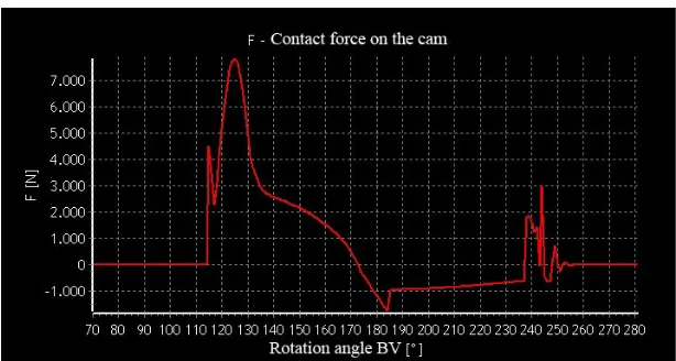
F1 is the contact force between the cam and the valve (later identified as FBV). It represents the main criterion for evaluation of valve train operation’s kinematic reliability.
The resultant of all vibration element forces according to Eq. (1) is (Eq. (6)):
(6)
Force F equals mass m inertia force (Eq. (7)): (7)
where is: [m/rad2] – is mass m (valve)
acceleration.
This is followed by the mass m motion differential equation (Eq. (8)):
(8)
When analyzing the measured cam, the lift function is defined by a set of points. Accordingly, the motion equation (Eq. (8)) cannot be solved analytically, but only numerically.
1. temporal integration of the motion equation is reduced to the initial value problem;
2. numeric finding of the distance function value based on function data in the past interval;
3. the problem with the stability and accuracy of the numeric methods used. Levy and Wilkinson (1976) presented a temporal integral method using as an additional requirement: acceleration at point 0. Namely, if h(t) is the distance of mass m, the 2nd derivation of is its
acceleration, so the 2nd Newton Law will
apply: , or (Eq. (9)):
By using the differentiation reversely:
and the Maclaurin formula, we derived the expressions for the 1st
derivation in the form of (Eq. (10)):
with queue
accuracy
with queue accuracy (10)
This method developed by Houbolt (1950), always converges and the temporal integration ∆ t step must be as follows to achieve good queue accuracy (Eq. (11)):
(11)
where is: ζmax [rad/s] – is the highest
internal circular vibration system vibrating
frequency; kmax [N/m] – is the stiffness of the strongest spring acting on mass m.
The initial requirements for integration are met if we assume that mass m is stationary at the beginning of the observed time interval (Eq. (12)):
(12)
5. Description of the Computational Tool
“MOTORI 2004”
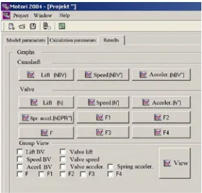
MOTORI 2004 is a windows-based application developed in a Borland Builder C++ 6.0 software environment, Croatian version. When starting the program i.e. opening a new project, a GUI interface opens, offering entry and modification of data displayed on the left side of the model design. Data may also be entered using a *.dvp file containing all input elements presented in Fig. 2a, and so may data for the tested cam profile throughout the 360° period. Two such files have been created for our two tested engine types, named motor-1. dvp and motor-2.dvp.
Fig. 2a.
Computing Tool Interface Presenting Model Parameters
Fig. 2b.
Computing Tool Interface Presenting Calculation Parameters
As is shown in Fig. 2c, it is possible to graphically
present individual camshaft parameters (Fig. 3), individual valve parameters, and to present valve parameters in aggregate (Fig. 4).
Fig. 2c.
Fig. 3.
Graphic Presentation of Individual Camshaft Parameters (Lift, Speed and Acceleration)
A pitch in the files for the tested cam profile is 1°, which provides the most accurate results in most tested methods for numeric derivation and also represents a good
Fig. 4.
Graphic Presentation of Camshaft Parameters (Lift, Speed and Acceleration) in Aggregate
6. Model Testing
For the purposes of testing valve train model’s dynamic response, two sets of stiffness and damping constants were developed, named
Motor-1 and Motor-2. Motor-1 (Mahalec, 1996), corresponds to a highly stiff valve train, for example in an engine with a camshaft in the cylinder head, located directly above
the valves with transmission of shift to the valve via shell lifters (for example, in the Fiat 128 A). On the other hand, Motor-2 is a representative of low-stiffness design, e.g. an engine with a camshaft in the cylinder block, long lifter rods and rocker arms (e.g. in air-cooled boxer engines in VW cars. Table 1 presents the stiffness and damping constants for these two engine sets.
Table 1
Stiffness and Damping Constants for Motor-1 and Motor-2
Symbol Motor-1 Motor-2
Camshaft in bearings
k1, kRM [kN/mm] 1,5×10⁵ 3,25×10⁵
c1, cRM [kg/s] 1200 100
ζ1 , ζRM 0,1 0,06
Valve spring
k2, kOV [N/mm] 38,2 30,4
c2, cOV [kg/s] 0,4 0,4
ζ2 , ζOV 0,002 0,002
Valve seat
k3, kSV [kN/mm] 1,8×10⁵ 1,8×10⁵
c3, cSV [kg/s] 4000 4000
ζ3 , ζSV 0,3 0,3
Valvesprings with adjacentthreads k4, kNN [kN/mm]c4, cNN [kg/s] 1,8×1054000 1,8×1054000
ζ4 , ζNN 0,3 0,3
The first symbol in Table 1 (e.g. k1) pertains
to the dynamic model (see Fig. 1), while the second one (kRM) is used in the presented
diagrams. Both symbols denote the same element, the valve train in this case.
Profile K1 is analytically defined through the Kurz cam (Kurz, 1954), which is almost identical to the profile of the contemplated Fiat 128 A engine.
It is first necessary to test the impact of the stiffness and damping constants on the contact force as the main indicator of the relation between the valve and the cam. In addition, we need to see the model’s response in different driving conditions i.e. clearance and rotational speed.
Testing determined that stiffness constant
kRM and damping constant cRM had the most
important impact, significantly affecting the vibration of the curve describing contact force variation across the camshaft twist angle.
If we look at Fig. 5, we will see the impact of valve train stiffness on the contact force on the cam. As we increase stiffness constant
kRM up to a certain limit (50 kN/mm), contact
force vibration decreases. If continues to increase and its value rises to, for example, 1000 kN/mm (see Fig. 6), contact force vibration increases intensively because the forces of camshaft’s bending in the bearings also grow. The cam hits against the valve, bounces off it and flies away for a brief time. We could say that an excessively stiff valve train acts like a hard bumper, like there is too little damping. The inertia force prevails in the contact force in such case. The simulation results are presented for Motor-1.
Fig. 5.
Fig. 6.
Contact Force on the Cam as a Result of Increase in Valve Train Stiffness to 1000 kN/mm (for Motor-1)
7. Conclusion and Future Research
The paper presents the MOTORI 2004
computing tool used for simulations and to present results of simulating cam profile dynamic responses. The presentation of the tool itself and the simulation results is preceded by a description of the valve train and in its mathematical presentation, with criteria set and implemented in the computing tool. The valve train is presented as a dynamic model with a single degree of freedom, where mass is restrained between 4 stopper-type vibration elements. The mathematical model enables us to temporally integrate the motion equations at a constant rotational speed over several consecutive camshaft revolutions. The simulation outputs are diagrams showing the distance, speed and acceleration of the camshaft and valves, forces of the respective vibration elements, the individually presented contact force on the cam, and the possibility of jointly displaying the individual values in a chart. Results may be displayed for a single rotational speed and
for a specific speed range, with the option of choosing pitches. The results of simulation at the valve opening point and in imaginary extreme operating conditions (soft/hard spring, low/high damping, low/high rotational speed and increased clearance) are tested and presented separately. The main criterion for evaluation of valve train’s dynamic behavior was the contact force between the cam and valve. Simulations were carried out for two engines of different designs.
As an extension to this research, we could propose expansion of the computing tool that will use computing methods to enable comparison between dynamic response simulation results and experimental results and evaluation of the cam profile’s operation as a result of wearing.
References
Carlini, A.; Rivola, A.; Dalpiaz, G.; Maggiore, A. 2002. Valve motion measurements on motorbike cylinder heads using high speed laser vibrometer. In Proceedings of the 5th International Conference on Vibration Measurements by Laser Techniques: Advances and Applications, Ancona, Italy, 564-574.
Choi, T.D.; Eslinger, C.T.; Kelley, O.J.; David, J.W.; Etheridge, M. 2000. Optimization of Automotive Valve Train Components with Implicit Filtering,
Optimization and Engineering. DOI: http://dx.doi. org/10.1023/A:1010071821464, 1(1): 9-27.
David, J.W.; Cheng, C.Y.; Choi, T.D.; Kelley, C.T.; Gablonsky, J. 1997. Optimal Design of High Speed Mechanical Systems, North Carolina State University, USA, Technical Report, CRSC-TR97-18.
De Wilde, E.F. 1967. Investigation of Engine Exhaust Valve Wear, Wear. DOI: http://dx.doi.org/10.1016/0043-1648(67)90007-5, 10(3): 231-244.
Derndinger, H.-O. 1959. Untersuchungen über das dynamische Verhalten der Ventile an Verbrennungsmotoren, PhD thesis, TH Karlruhe, Germany.
Dujmović, L.; Kozarac, D.; Lulić, Z. 2005. Numerical Simulation of Valve Train Dynamics. In Proceedings of the 10th EAEC European Automotive Congress, Belgrade, Serbia.
Hafner, K.E. 1973. Investigating the Dynamic Behavior of Valve Mechanisms with Engineering Vibration Methods. In Proceedings of 10th International Congress Combustion Engines, New York, USA, 313-337.
Houbolt, J.C. 1950. A recurrence matrix solution for the dynamic response of elastic aircraft, Journal of Aeronautical Sciences, 17(9): 540-550.
Jeon, H.S.; Park, K.J.; Park, Y.-S. 1989. An Optimal Cam Profile Design Considering Dynamic Characteristics of a Cam valve System, Experimental Mechanics. DOI: http://dx.doi.org/10.1007/BF02323851, 29(4): 357-363.
Kim, W.J.; Jeon, H.-S.; Park, Y.S. 1991. Contact Force Prediction and Experimental Verification on an OHC Finger-follower type Cam valve System,
Experimental Mechanics. DOI: http://dx.doi.org/10.1007/ BF02327568, 31(2): 150-156.
Kurz, D. 1954. Entwurf und Berechung ruckfreier Nocken, ATZ, 11: 293-299.
Levy, S.; Wilkinson, J.P.D. 1976. The Component Element Method in Dynamics, McGraw-Hill, USA.
Mahalec, I. 1996. The Dynamic Response of Valve Train due to the Cam Profile Errors, (in Croatian), PhD thesis, FMENA Zagreb, Croatia.
McAlpine, H.; Hicks, B.J.; Huetand, G.; Culley, S.J. 2006. An investigation into the use and content of the engineer’s logbook, Design Studies. DOI: http://dx.doi. org/10.1016/j.destud.2005.12.001, 27(4): 481-504.
Plötzner, R.; Lowe, R. (Eds.) 2004. Special Issue: Dynamic visualizations and learning, Learning and Instruction, 14: 235-357.
Schrick, P. 1969. Über das dynamische Verhalten von Ventilsteuerungen an Verbrennungsmotoren, PhD thesis, TU Carolo-Wilhelmina zu Braunschweig, Germany.
Teodorescu, M.; Kushwaha, M.; Rahnejat, H.; Taraza, D. 2012. Elastodynamic transient analysis of a four-cylinder valve train system with camshaft flexibility. In Proceedings of the Institution of Mechanical Engineers, Part D: Journal of Automobile Engineering, 226(1): 94-111.
Tounsi, M.; Chaari, F.; Walha, L.; Fakhfakh, T.; Haddar, M. 2011. Dynamic behavior of a valve train system in presence of camshaft Errors, WSEAS Transactions on Applied and Theoretical Mechanics, 6(1): 17-26.