Complete Graph Technique Based Optimization In Meadow Method Of Robotic Path Planning

(1)

Complete Graph Technique Based

Optimization In Meadow Method Of Robotic

Path Planning

S. Singh*,G. Agarwal#

* Dept. of Information technology ,Invertis Institute Of Engineering and technology, Bareilly (UP) ,India # Dept. of computer science, Invertis Institute Of Engineering and technology, Bareilly (UP) ,India

[email protected](S Singh),[email protected](G.Agarwal)

Abstract: This paper explores new dimension in optimal path planning, Here we are proposing a new algorithm ‘OPTIMIZED PATH PLANING ALGORITHM’, which optimizes the path between single source to single destination. The proposed algorithm optimizes the path found by Dijkstra’s algorithm, it is proven in this paper that the new path is better than the path found by Dijkstra’s algorithm. The simulator is developed in C- language, on the basis of which, comparison table has been constructed which shows better performance of the proposed algorithm. First step is Object Growing in which the object is grown to its configuration space and produces the actual space for robot navigation. Next step is possible complete graph generation, in which a graph is drawn connecting all the obstacles, this is a complete graph and better than those of convex polygon graph in Meadow Maps technique as it has more edges producing more information. Mid point network generation, connects the midpoints of all these edges and creates the path for robot movement. Then we find a path using Dijkstra’s algorithm [8], the best in single source and single destination problems. We applied our algorithm “Optimized Algorithm” and hence creating a more optimized path, which is approximate to ideal path, consist of less turns and hence saves energy.

Keywords: Complete Graph Method, Meadow Method Optimization, Dijkastra’s Optimized Path.

1. Introduction

Path planning is an open robotic problem. The problem can be stated as “ How to find a path in a work space with obstacles from a start point to a goal point which is most efficient in term of length of the path and energy consumed by robot in getting goal.”

Following are previously used terms and techniques in the field of robot navigation. Each technique has its own advantages and disadvantages. We are showing here the main techniques (Some Terms and Methods) which are being used till now (previous work) .

• Configuration space [9] • Generalized Voronoi graphs [9] • Grids based motion planning[8] • Graph-based planners: A* [8] • Meadow maps

1.1. Configuration Space [9]

1.1.1. Configuration Space [9] (abbreviated: “C-space”):

(2)

1.2. Generalized Voronoi graphs

• Steps involve creation of voronoi edge. • Voronoi edge is equidistant from all points. • Points where these edges meet is voronoi vertex.

1.2.1. Basic GVG approach:

Generate a Voronoi edge, which is equidistant from all points. Point where Voronoi edge meets is called a Voronoi vertex. Vertices often have physical correspondence to aspects of environment that can be sensed If robot follows Voronoi edge, it won’t collide with any modeled obstacles.

1.3 Grids

a) Superimposes a 2D Cartesian grid on the world space.

b) If there is any object in the area contained by a grid element, that element is marked as occupied. c) Center of each element in grid becomes a node, leading to highly connected graph.

d) Grids are either considered 4-connected or 8-connected.

Fig-1 Grid based Technique 1.4. Graph-based planners:

• Path finding between initial node and goal node can be done using graph search algorithms (Dijkastra’s Algorithm is one of the best algorithms used for this purpose) .

• However, many graph search algorithms require visiting each node in graph to determine shortest path - Computationally tractable for sparsely connected graph (e.g., Voronoi diagram) - Computationally expensive for highly connected graph (e.g., regular grid)

• Therefore, interest is in “branch and bound” search - Prunes off paths that aren’t optimal

• Classic approach: A* search algorithm

- Frequently used for holonomic robots

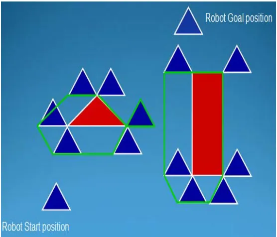
1.5) Meadow maps

• Transform space into convex polygons

– Polygons represent safe regions for robot to traverse

• Important property of convex polygons:

– If robot starts on perimeter and goes in a straight line to any other point on the perimeter, it will not go outside the polygon

• Path planning:

(3)

Following are the steps involved in Meadow Method- 1. Grow objects (explained below).

2. Construct convex polygons.

3. Mark midpoints; these become graph nodes for path planner. 4. Path planner plans path based upon new graph.

Fig. 2 Meadow Map method

2. Optimized Meadow Method: The Proposed Algorithm 2.1. The Concept

The Method has been divided in to different modules, each one for a specific task.. 2.1.1 The Block Diagram:-

(4)

2.2. The Proposed Technique - Optimized Algorithm -

2.2.1. Object Growing

This is the process of enlargement of obstacles by moving the robot around each obstacle using one reference point on robot’s boundary. The reference point can then be considered as robot itself and area swapped by the robot is added restricted area in the work space. It can be seen from the fig- 4 that there is a fix robot start position as well as robot’s goal position (shown in BLUE color) and obstacles (shown in RED color) which robot has to avoid in the process of navigation.In the fig. 4 object growing is shown. This shows the actual area in which robot will move in order to avoid the obstacles. After object growing, robot can be considered as a point with left most corner, and a region has been specified in which robot can not move. This process is called object enlargement where it seems that the size of object has grown.

2.2.2. Complete graph generation

A complete graph is created using the corners of obstacles. In this figure black lines are objects which are surrounded by gray boundaries(Enlarged area).

(5)

Fig 5 – Complete Graph Generation

2.2.3. Mid point network generation:

After complete graph generation, we get- Mid point of each edge (no. of midpoints will be less than or equal to number of edges in the complete graph.) These midpoints will be fixed for that particular problem. Start and goal position may vary according to input of user. for start and goal we need two more nodes. Total number of nodes in possible mid point network is less than or equal to 2 plus the number of edges in the complete graph.

Fig. 4 – Mid point Network Generation

2.2.4. Path finding

(6)

Fig. 5 – Applying Dijkstra’s Algorithm

2.2.5. Path Optimization

For path optimization we have developed the following algorithm , this algorithm gets a path which is approximately ideal path. This also reduces the number of turns which saves energy. The path in CYAN color is the path after applying Optimized Algorithm. Which is close to ideal path i.e. in Blue dotted color. The algorithm takes dijkastra’s path between source and destination as reference and works as follows- real_initial_position (Source) and real_goal_position (Destination) are duplicated in temp_initial_position and temp_goal_position. If temp_initial_position and temp_goal_position are not visible to each other ( There is any part of obstacle between them) than temp_goal_position is assigned the node coming earlier to the current node in temp_goal_position on dijkastra’s path. But if temp_initial_position and temp_goal_position are visible to each other ( There is no part of obstacle between them) than temp_goal_position is added to the optimized path skipping the nodes coming between temp_initial_position and temp_goal_position on dijkastra’s path (Next_node array is used for this purpose) and temp_initial_position is shifted to temp_goal_position and temp_goal_position is assigned real_goal_position. This process is repeated until compete optimized path is found.

(7)

2.3 ALGORITHM : Optimization of path obtained by Dijkastra’s algorithm

1. Select Real_Initial_Position And Real_Goal_Position;

2. a) temp_Initial_Position  Real Initial Position b) temp_Goal_Position  Real_Goal_Position

c) Next_Node [0] temp_Initial_position; Add=1;// Add is array index

3. If(PathExists Between temp_Initial_Position and temp_Goal_Position) {

temp_Initial_Position temp_Goal_Position; temp_Goal_Position  Real_Goal_Position; Next_Node[add++]  temp_Initial_Position;

IF( temp_Initial_Position=Real_Goal_Position)

Then GoTo step 4. Else

GoTo step 3. }

Else {

temp_Goal_PositionPrevious Node Exists On Reference Dijkastra’s Path;

}

4. STOP.

3. Comparative Analysis:

3.1. Displaying Results

Following is a comparison chart (Table 1) between Dijkstra’s algorithm and Optimize algorithm. This chart has been created on the basis of 13 run of simulator by taking different cases of start and goal positions and different obstacles positions, shapes and sizes. In every case optimized path was better than Dijkastra’s algorithm. Problem Dijkastra’s Path length Optimized Path Length Optimization Turns In dijkastra’s Path Turns In Optimized Path Result

Problem 1 547 547 0 0 0 Both are equal

Problem 2 320 320 0 0 0 Both are equal

Problem 3 619 526 93 2 2 Opt. is Better

(8)

5. Advantages Of Technique

 Optimize Tech. always gives better path with less distance.  Optimize tech. gives less zigzag path with less and genuine turns.  Less turns helps Robot for Energy & Time saving.

 Very good for both from simplest one to complex one.

6. Limitations Of Technique

This technique can not work with curved shape Map. As it has been designed specifically for rectangular, triangular, squared obstacles.

7. Conclusion

 Optimize Technique approach is better than convex Polygon based Meadow map technique.

 Optimize Technique path may be less efficient than Ideal path but Optimal Path always better than Single Dijkastra’s Path.

8. References

[1] Brooks, R., Cambrian Intelligence: The Early History of the New AI, MIT Press, 1999. [2] Brooks, R., and Flynn, A., Fast, Cheap and Out of Control, AI Memo 1182, MIT [3] Elaine Rich and Kelvin Knight,Artificial Intelligence,T.M.H,2000.

[4] G. van den Bergen, Collision detection in interactive 3D computer animation, PhD thesis, Eindhoven University, 1999. [5] Hanna Kurniawati, Work Space Based Sampling for Probabilistic Path Planning, Ph.D. Thesis,School of computing,

National University of Singapore, 2007.

[6] Lozano-P´erez and M. Wesley. An algorithm for planning collisionfree paths among polyhedral obstacles. Comm. ACM, 22(10):560–570, 1979.

[7] Robin R. Murphy ,Introduction to AI Robotics,MIT Press,2000. AI Laboratory, December, 1989.

[8] Roland Jan Geraerts,Sampling-based Motion Planning : Analysis and path Quality, Ph.D. Thesis,Utrecht University,2006 [9] Subramanian Ramamoorthy, Task Encoding,Motion Planningg and Intelligent Control using Qualitative Models, Doctor of

Philosophy Dissertation, University of texas,Austin,2007.