Information and the dynamics of SEIR
e-epidemic model for the spreading behavior
of malicious objects in Computer Network
Radha Tamal Goswamia, Bimal Kumar Mishrab
a
Department of Computer Science and Engineering, Birla Institute of Technology, Mesra, Kolkata Campus, Kolkata, India – 700 107
Email: [email protected]
b
Department of Applied Mathematics, Birla Institute of Technology, Mesra, Ranchi, India – 835 215 Email: [email protected]
Abstract
An e – epidemic model has been developed with optimal shelter for malicious objects in computer network. We first find the basic reproduction number and study the malicious code free equilibrium which concludes that whether the malicious objects invade the network or dies out. By using MATLAB and numerical methods, we give some numerical simulations in the support of our mathematical conclusions which show the stability of the system of differential equations developed.
Key – Words
Stability; Basic Reproduction Number; Equilibrium; Malicious Codes 1. Introduction
Today in the modern age of science and technology, Electronic mail and use of secondary devices are the major responsible sources for the transmission of malicious objects in computer network [1]. Malicious object is a code that infects computer systems. It is a computer program that operates on behalf of a potential intruder to aid in attacking a system or network. Historically, an arsenal of such agents consisted of viruses, worms, and trojanized programs and by combining key features of these agents, attackers are now able to create software that poses a serious threat even to organizations that fortify their network perimeter which is protected with firewalls and other defensive materials. In a certain sense, the propagation of virtual malicious objects in a system of interacting and integrated computers could be compared with a disease transmitted by vectors when dealing with public health. Concerned diseases transmitted by vectors, one has to take into account that the parasites spent part of its lifetime inhabiting the vector, so that the infection switches back and forth between host and vector.
Based on epidemiological models proposed by Kermack and Mckendrics [2 – 4], the attacking and spreading behavior of malicious codes in a computer network can be studied by using the different e - epidemic models given by Mishra et al [5 - 10]. Richard and Mark [11] propose an improved model to simulate virus propagation.
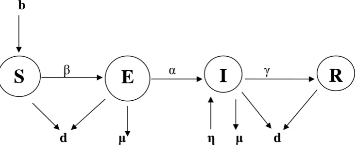
2. Formulation of the Model
Figure 1:Schematic diagram for the flow of malicious codes in computer network.
The transmission between model classes can be expressed by the following system of differential equations:
b
SI
dS
dt
dS
SI
d
E
dt
dE
)
(
E
d
I
dt
dI
)
(
(1)
I
dR
dt
dR
Where, b is the birth rate (new nodes attached to the network), d is the natural death rate (that is, crashing of the nodes other than the attack of malicious codes), βSI is the incidence of malicious code infection and β is the rate of contact (that is, from class S to class E), α is the rate of transmission from class E to class I, γ is the rate of recovery from class I to class R, μ is the death-rate (crashing of the nodes) due to the attack of malicious codes. The model also assumes that the flow of malicious codes between the classes can be spread through vertical transmission. In this case, the attack of malicious codes through vertical transmission increases at the rate η and is introduced at the class I. In this model, the flow of malicious codes is from class S to class E, class E to class I, class I to class R.
We now assume that our anti – virus software with latest signature is fully effective for optimal shelter. So, we introduce another parameter δ which is the shelter coverage rate of the susceptible computers. Then the system (1) becomes,
b
SI
dS
S
dt
dS
SI
d
E
dt
dE
)
(
E
d
I
dt
dI
)
(
(2)
I
dR
S
dt
dR
S
E
I
R
b
β
α
γ
where, ρ is any positive constant and M is information variable [12, 13] and summarizes information about both the current and past state of the virus infection, i.e. ܯdepends on current and past values of state variables. Then,
tg
S
t
I
t
K
t
d
M
(
(
),
(
))
(
)
where, K is the delaying kernel [14] and τ is the distributed delay, which means susceptible individuals S and infective individuals Iare affected at time tby the state variables Sand I at possibly all previous time ߬. Other variables are given by:
(1) According to the assumptions that the shelter coverage depends on both past and present incidence of infection, then it is easy to take, g (ܵ, ܫ) = ߚܵܫ.
(2) We also take,
T
T
t
t
K
)
(
exp
)
(
[15], where, T is positive constant and representingthe average delay of collected information of infection.
From these two assumptions, the model (2) can be re – written as,
b
SI
dS
MS
dt
dS
SI
d
E
dt
dE
)
(
E
d
I
dt
dI
)
(
(4)
I
dR
MS
dt
dR
1
(
SI
M
)
T
dt
dM
3. Solution and Stability
In this section, we analyze the malicious codes-free equilibrium and get the basic reproduction number for the malicious codes control or eradication. Since the class R is not present in the rest of the equations in system (4), that is, the analysis will be restricted the dynamics of the four equations of the system (4).
b
SI
dS
MS
dt
dS
SI
d
E
dt
dE
)
(
E
d
I
dt
dI
)
(
(5)
1
(
SI
M
)
T
dt
dM
Thus,
d
b
U = { (S, E, I, M) : S, E, I, M ≥ 0, S + E + I + M ≤
d
b
} is a positive invariant set for the model. In the absence
of infection, the model has a unique malicious codes - free equilibrium, P0 (
d
b
, 0, 0, 0) and an endemic
equilibrium P* (S*, E*, I*, M*), where, the points can be obtained by taking,
E
I
M
S
0
(from system(5)), as,
0
*
1
R
S
,)
(
)
)(
(
0 0 0 *
R
d
bR
d
R
E
,)
(
)
(
0 0 0 *
R
d
bR
R
I
,
0 0 *R
d
bR
M
Where, R0 is basic reproduction number can be obtained by taking 2nd and 3rd equations of system (5) and after
linearization, we get,
I
E
V
F
I
E
(
)
, where, F and V can be defined as,
0
0
0
F
and
d
d
V
0
Then R0 is the dominant eigenvalue of F V-1. That is,
)
)(
(
0
d
d
R
.Now, for locally asymptotically stable, we define the Jacobian of the system (5), as,
T
d
d
d
J
1
0
0
0
0
)
(
0
0
0
)
(
0
0
0
0
(6)The eigenvalues of this matrix are, - d, - (d + μ + α), - (d + μ + γ – η), - 1/T. Since all the eigenvalues are negative, then the malicious – codes free equilibrium is locally asymptotically stable. Thus we can get the following results:
Lemma 1: If R0 < 1, the malicious – codes free equilibrium P0 is locally asymptotically stable, whereas, if R0 > 1,
P0 is unstable.
Lemma 2: If R0 > 1, the endemic equilibrium P* is locally asymptotically stable.
Proof: Lemma 1 is quite obvious from above discussion. For lemma 2, by using the system (5) and equation (6), the characteristic equation will be,
0
4 3 2 2 3 1 4
a
+
λ
a
+
λ
a
+
λ
a
+
λ
If λi (i = 1, 2, 3, 4) are the roots of this equation, then, a1 = λ1, a2 = λ1λ2, a3 = λ1λ2λ3, a4 = λ1λ2λ3λ4
satisfying Hurwitz’s condition which tells that, a1 > 0, a2 > 0, a3 > 0, a4 > 0 and a1a2a3 - a32 - a12a4 > 0.
So, the endemic equilibrium P* is locally asymptotically stable. 4. Numerical Discussion and Conclusion
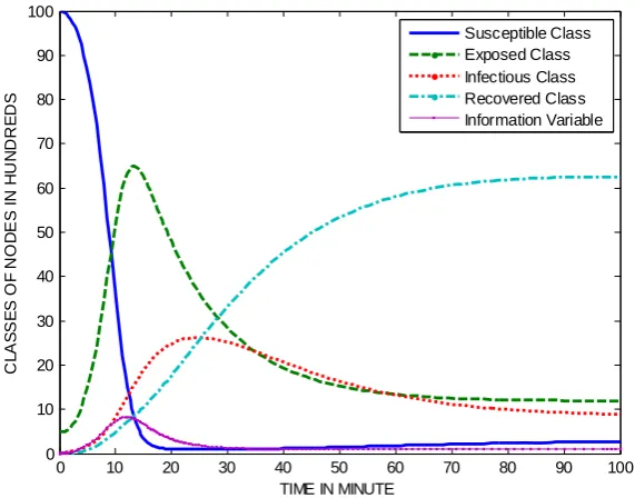
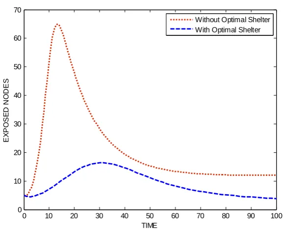
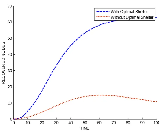
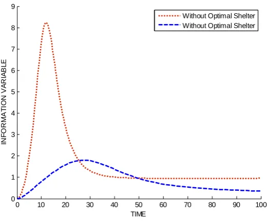
Analysis and simulation results show some managerial insights that are helpful for the practice of antivirus in information sharing networks. Figure - 1 shows the behavior of different classes of nodes without optimal shelter while figure – 2 represents the same with optimal shelter using information variable which leads the stability of the system. A comparison between with and/or without optimal shelter is analyzed among the different classes of nodes and information variable which shows that it is necessary to set optimal shelter coverage to keep malicious – codes away from propagation (depicted in figures 3 – 7).
Figure 1: Dynamical behavior of the system (1) without information variable with real parametric values, b = 1, β = 0.05, μ = 0.05, γ = 0.07,
α = 0.05, d = 0.01, η = 0.03.
Figure 2: Dynamical behavior of the system (4) with information variable and real parametric values, b = 1, β = 0.04, μ = 0.02, γ = 0.07, α = 0.05, d = 0.01, η = 0.03, ρ = 0.002, T = 5.
0 10 20 30 40 50 60 70 80 90 100
0 10 20 30 40 50 60 70 80 90 100
TIME IN MINUTES
C
L
AS
SE
S
O
F
NO
D
E
S
I
N
H
UN
D
RE
D
S
Susceptible Exposed Infectious Recovered
0 10 20 30 40 50 60 70 80 90 100
0 10 20 30 40 50 60 70 80 90 100
TIME IN MINUTE
CL
AS
SE
S
O
F
NO
D
E
S
I
N
H
U
N
DRE
DS
Figure 3: Dynamical behavior of susceptible class
Figure 4: Dynamical behavior of exposed class
0 10 20 30 40 50 60 70 80 90 100
0 10 20 30 40 50 60 70 80 90 100
TIME
SU
SC
E
P
TI
BL
E N
O
D
E
S
With Optimal Shelter Without Optimal Shelter
0 10 20 30 40 50 60 70 80 90 100
0 10 20 30 40 50 60 70
TIME
EX
PO
SE
D
NO
D
ES
Figure 5: Dynamical behavior of infectious class
Figure 6: Dynamical behavior of recovered class
0 10 20 30 40 50 60 70 80 90 100
0 5 10 15 20 25 30
TIME
IN
F
E
C
T
IO
U
S
N
O
D
E
S
Without Optimal Shelter With Optimal Shelter
0 10 20 30 40 50 60 70 80 90 100
0 10 20 30 40 50 60 70
TIME
RE
CO
V
E
RE
D
N
O
D
E
S
Figure 7: Dynamical behavior of information variable
References:
[1] M.E.J. Newman, Stephanie Forrest, Justin Balthrop, Email networks and the spread of computer viruses, Phys. Rev. E 66 (2002) 035101–035104.
[2] W. O. Kermack, A. G. Mckendrick, Gontributions of mathematical theory to epidemics, Proceeding of the Royal Society of London-Series A, 115 (1927), 700-721
[3] W. O. Kermack, A. G. Mckendrick, Gontributions of mathematical theory to epidemics, Proceeding of the Royal Society of London-Series A, 138 (1932), 55-83
[4] W. O. Kermack, A.G. Mckendrick, Gontributions of mathematical theory to epidemics, Proceeding of the Royal Society of London-Series A, 141 (1933), 94-122
[5] Bimal Kumar Mishra and D. K. Saini, SEIRS epidemic model with delay for transmission of malicious objects in computer network, Applied Mathematics and Computation, 188 (2) (2007), 1476-1482.
[6] Bimal Kumar Mishra and Dinesh Saini, Mathematical models on computer viruses, Applied Mathematics and Computation, 187 (2) (2007), 929-936
[7] Bimal Kumar Mishra and Navnit Jha, Fixed period of temporary immunity after run of anti-malicious software on computer nodes, Applied Mathematics and Computation, 190 (2) (2007) 1207 – 1212.
[8] Bimal Kumar Mishra, Samir Kumar Pandey. Dynamic Model of worms with vertical transmission in computer network. Applied Mathematics and Computation. 2011, Volume 217, Issue 21, pp 8438-8446
[9] Samir Kumar Pandey, Bimal Kumar Mishra, P. K. Satpathy, A Distributed Time Delay Model of Worms in Computer Network, CiiT International Journal of Networking and Communication Engineering, 3 (6), 2011, pp. 441 – 447.
[10] Bimal Kumar Mishra, Samir Kumar Pandey, Fuzzy epidemic model for the transmission of worms in computer network, Nonlinear Analysis: Real World Applications, 11, 2010, pp. 4335-4341.
[11] W.T. Richard, J.C. Mark, Modeling virus propagation in peer-to-peer networks, in: IEEE International Conference on Information, Communications and Signal Processing (ICICS 2005), pp. 981–985.
[12] A. d’Onofrio, P. Manfredi, E. Salinelli, Vaccinating behaviour, information and the dynamics of SIR vaccine printable diseased, Theoretical Population Biology, 71 (2007), 301-307
[13] A. d’Onofrio, P. Manfredi, E. Salinelli, Bifurcation thresholds in a SIR model with information dependent vaccination, Mathematical Modelling of Natural Phenomena, Epidemiology, 2(1), 2007, 26-43
[14] J. Guckenheimer, P. Holmes, Nonlear Oscillations, Dynamical Systems, and Bifurcations of Vector Fields, Springer-Verlag, New York, 1983, 117-156
[15] T. K. Kar, P. K. Mondal, Global dynamics and bifurcation in delayed SIR epidemic model, Nonlinear Analysis: Real World Application, Volume 12, Issue 4, August 2011, 2058-2068
0 10 20 30 40 50 60 70 80 90 100
0 1 2 3 4 5 6 7 8 9
TIME
IN
F
O
RM
A
T
IO
N V
A
RI
A
B
L
E