Parallel Simulation of Queueing Petri Nets

(1)

Parallel Simulation of Queueing Petri Nets

Jürgen Walter

University of Würzburg 97074 Würzburg Germany

Simon Spinner

Samuel Kounev

ABSTRACT

Queueing Petri Nets (QPNs) are a powerful formalism to

model the performance of software systems. Such

mod-els can be solved using analytical or simulation techniques. Analytical techniques suﬀer from scalability issues, whereas simulation techniques often require very long simulation runs. Existing simulation techniques for QPNs are strictly sequen-tial and cannot exploit the parallelism provided by modern multi-core processors. In this paper, we present an approach to parallel discrete-event simulation of QPNs using a con-servative synchronization algorithm. We consider the spa-tial decomposition of QPNs as well as the lookahead cal-culation for diﬀerent scheduling strategies. Additionally, we propose techniques to reduce the synchronization over-head when simulating performance models describing sys-tems with open workloads. The approach is evaluated in three case studies using performance models of real-world software systems. We observe speedups between 1.9 and 2.5 for these case studies. We also assessed the maximum speedup that can be achieved with our approach using syn-thetic models.

Keywords

Parallel discrete eventsimulation, performance prediction, stochasticperformance modeling,queueingpetrinets

1. INTRODUCTION

Queueing Petri Nets (QPNs) are a combination of Colored Generalized Stochastic Petri Nets (CGSPNs) [6] and Queue-ing Networks (QNs) [20]. In [23], the authors show the ben-eﬁts of using QPNs in terms of modeling power and expres-siveness when analyzing the performance behavior of soft-ware systems. In contrast to traditional QNs and CGSPNs, QPNs enable the description of hardware and software as-pects of system behavior in the same model [23]. Software contention eﬀects, such as synchronization, simultaneous re-source possession and blocking, can be easily described us-ing QPNs [23]. In recent years, QPNs have been successfully

used to model the performance of diﬀerent types of software systems (e.g., component-based systems, event-based sys-tems, database syssys-tems, computer networks, or multi-tenant systems [22, 38, 34, 37, 39], see1 for more). The respective case studies use QPN models for the quantitative analysis of the performance and the scalability of a system under test. QPN models can be analyzed quantitatively using analyti-cal or simulation-based solution techniques. Analytianalyti-cal so-lution techniques for QPNs are based on transformations to Markov chains. However, models of realistic software sys-tems often result in Markov chains with a too large state space to be analytically tractable [23]. In contrast, simu-lation techniques provide better scalability and thus enable the analysis of models that could not be solved analytically. SimQPN, which is part of the Queueing Petri Net Modeling Environment (QPME) [42, 24], is the only discrete-event simulator for QPNs currently available. However, the im-plementation of SimQPN is strictly sequential, limiting its performance on modern multi-core computer systems.

Diﬀerent approaches to parallel discrete-event simulation have been proposed in the literature to leverage the poten-tial speedup of modern multi-core computer systems [15]. While the general challenges of parallelizing a discrete-event simulation are well understood, the actual speedup heav-ily depends on the characteristics of the used modeling for-malism and the concrete model. So far, only the authors of [18] have evaluated the potential speedup for QPNs using parallel event-discrete simulation. However, this work does not consider queueing places and their associated schedul-ing strategies, which are an integral part of QPNs (e.g., to model hardware contention eﬀects in a system). The choice of scheduling strategies can severely impact the paralleliza-tion potential of discrete-event simulaparalleliza-tion, as shown in [27] for traditional QNs.

Novel use cases of QPNs identified in the last few years require substantial improvements in simulation speed. The first scenario is online performance prediction for run-time resource management. Many software systems are subject to Service Level Agreements (SLAs) regarding response time or throughput. In order to proactively reconfigure a system before SLAs are violated, it is necessary to be able to predict the system performance under different configurations and workloads. QPNs provide the modeling power and expres-siveness required for such performance predictions. In online performance prediction scenarios [8], the time for solving QPNs models is a limiting factor in order to be able to react before SLAs are violated. Speedups through parallel

simu-1_{https://go.uni-wuerzburg.de/qpnbibliography}

(2)

lation would enable the timely analysis of larger and more accurate models. The second scenario is the use of QPNs to analyze design-orientedarchitecture-level performance mod-els, which describe a system with a high level of detail. In [28], the authors propose a transformation from the Palla-dio Component Model (PCM) [7] to QPNs for performance analysis. Applied to practical PCM models, the transforma-tion often results in large and complex QPNs models [28]. A signiﬁcant speedup of simulation speed is especially worth-while for such models. Given that the number of cores of modern processors is continuously increasing while the clock frequency stays the same, parallel simulation techniques can provide the speedup required by the previously described us-age scenarios for QPNs. In this paper, we show how parallel simulation techniques can be applied to analyze QPNs and evaluate the potential speedup of QPN simulation through parallelization. More speciﬁcally, we make the following con-tributions:

1. We explore the potential of QPNs for parallel event-discrete simulation, which includes the analysis of looka-head estimation for QPNs.

2. We propose a Directed Acyclic Graph (DAG) decom-position approach for QPNs required for eﬃcient par-allel discrete-event simulation.

3. We provide an implementation of a parallel discrete-event simulation engine for QPNs based on the SimQPN simulation engine.

The evaluation of our approach is focused on the following two questions: 1) What speedup can be achieved by using discrete-event simulation for QPN models of realistic sys-tems? 2) What is the maximum speedup that can be prac-tically reached? To answer the ﬁrst question we conducted three case studies using performance models of real-world systems: a model of a large Software-as-a-Service (SaaS) provider, a model of a complex J2EE application, and a model describing the performance behavior of a data-center network. We observed speedups between 1.91 and 2.45 for the considered models. To answer the second question, we used a synthetic model to systematically benchmark the par-allel simulation. With the synthetic model, we could even observe super-linear speedups.

The remainder of this paper is organized as follows. We start with a brief introduction to the QPN formalism in Section 2 and parallel simulation in Section 3. Section 4 dis-cusses challenges for parallelization of discrete-event QPN simulation and presents the parallelization approach

includ-ing our assumptions and design decisions. Section 5

de-scribes the case studies. Section 6 is about related work. Section 7 concludes the paper.

2. QUEUEING PETRI NETS

Queueing Petri Nets (QPNs) are an extension of Colored Generalized Stochastic Petri Nets (CGSPNs) [24], a special type of Petri Nets (PNs). PNs are a general formalism for the analysis of concurrent systems. In mathematical terms, a PN is a directed bipartite graph with two diﬀerent types of nodes namedplaces and transitions. Places represent

sys-tem states and can contain a number of tokens. Tokens

can be used to represent resource availability, jobs to be ex-ecuted, ﬂow of control or synchronization conditions [32].

Theinitial markingcan be changed by theﬁring of transi-tions. Transitions are connected to input and output places

with forward and backwardincidence functions. The ﬁring

of a transition changes the system state by removing one token from each input place and adding one token to each output place. While PNs are easy to understand and have a rigorous mathematical foundation, PNs of realistic systems quickly become very large. Therefore, extensions to PNs have been proposed to improve its model expressiveness.

Jensen [17] describes Colored Petri Nets (CPNs) introduc-ing token colors which can be used to distintroduc-inguish between diﬀerent types of requests in a system. Firing modes can

be deﬁned depending on token colors. A color function C

assigns the diﬀerent ﬁring modes to transitions. The greater modeling convenience comes along with no loss of PN prop-erties since CPNs are a backward-compatible extension to

the original PNs. In addition to immediate transitions,

Generalized Stochastic Petri Nets (GSPNs) introducetimed

transitions enabling the integration of temporal aspects by assigning firing delays to transitions. The firing delay spec-ifies the time an enabled transition waits before it fires. If multiple timed transitions are enabled at the same time, the next transition to fire is chosen based onfiring weights

(probabilities) assigned to the transitions [26]. The combina-tion of CPNs and GSPNs results in CGSPNs [6]. CGSPNs are a powerful modeling formalism for describing concur-rency and synchronization aspects. However, CGSPNs do not support a direct representation of scheduling behaviors [4, 25] and therefore are limited when modeling hardware

contention [21]. The Queueing Petri Net (QPN)

formal-ism combines the advantages of QNs and PNs by

intro-ducing queueing places. A token that arrives at a

queue-ing place is first served in a queue (see QNs), before it is put in the depository. Only tokens in the depository are available to outgoing transitions. Queueing places enable the description of scheduling aspects in QPNs. QPNs are suited for quantitative, as well as qualitative analyses. In this paper, we focus on the quantitative analysis of QPNs required for the performance analysis of computer systems. The HiQPN tool [5] enables the analytical solution of QPNs. However, it is severely limited by the model size that can be solved [23]. SimQPN [24, 42] is a discrete-event sim-ulator for QPNs. SimQPN supports different methods for steady-state analysis (batch means, replication deletion, and method of Welch) and provides great flexibility in controlling the amount of quantitative data (e.g., utilization, through-put, and response time) collected for each place in a QPNs. SimQPN has been shown to scale well with increasing mod-eling size [28, 8]. However, SimQPN is currently a strictly sequential program and cannot utilize the parallelism offered by modern systems.

3. PARALLEL SIMULATION

(3)

be performed at the following three levels [19]:

• At theapplication level, replicated simulation runs can be executed in parallel. Replicated simulation runs are often used for variance reduction of a long simulation run by running multiple shorter runs or for investi-gating a large number of diﬀerent parameter settings [15]. This parallelization approach works well indepen-dently simulated model.

• At a functional level, individual functions (e.g., event list manipulation and random number generation) can be executed in parallel to the main simulation thread. In order to achieve significant speed-ups, this paral-lelization approach requires computationally expensive functions [15]. However, such functions are often an indicator for an inefficient implementation where opti-mization offers more potential than parallelization[18].

• At the event level, a simulated model can be decom-posed in spatial or temporal partitions. Each partition can be executed in its own process. In order to ensure the causal ordering of events, a synchronization be-tween the processes is required.

In this paper, we will focus on event-level parallel simu-lation QPNs, as this approach promises to provide advan-tages when simulating large models. By decomposing a large QPNs into smaller partitions, the overall simulation time may be reduced signiﬁcantly.

For an event-level parallel execution of a single simula-tion run several design quessimula-tions need to be answered. We need to decide on: model decomposition, synchronization algorithm (conservative vs. optimistic), and communication mode (synchronous vs. asynchronous). In the following, we give a short overview of diﬀerent techniques typically used for event-level parallel simulation. A detailed introduction to the topic can be found in [15].

Model decomposition: Parallel discrete-event

simula-tion decomposes the simulasimula-tion model into disjunct parti-tions, which are simulated in parallel. The corresponding process that executes the events within a single partition is called logical process (LP). The decomposition goal is to keep the load between LPs balanced while minimizing the communication costs. The decomposition is either spa-tial or temporal. Temporal decomposition requires (rarely available) knowledge about future system states to achieve speedup. Spatial decomposition partitions the net into sev-eral connected subnets. It scales with model size and of-fers more potential for speedup than temporal decomposi-tion [33].

Synchronization algorithm: The event processing of

the simulation is executed in an event loop in each LP. Hence, each LP has its dedicated virtual simulation time. In order to guarantee the local causality constraint (i.e., each LP processes events in nondecreasing timestamp or-der), timestamps need to be exchanged between LPs. For a correct causality of the simulation, synchronization algo-rithms are required to ensure that no token with a smaller timestamp than the LP’s current time may arrive later in the simulation. Conservative synchronization enforces the local causality constraint at every point in time. They pause processing if they reach a lookahead border waiting for the other LPs to progress further. Lookahead is the (virtual)

time span from the current clock for which an LP is guaran-teed to receive no incoming events with smaller timestamps from neighboring LPs. It is the time an LP can process without synchronization. The largest possible lookahead is the time interval an LP has from the current clock time un-til processing of the next incoming token. Often lookahead estimation in conservative approaches is far from optimal. The predicted lookahead is less than the maximum possi-ble lookahead. In the worst case, the predicted lookahead is zero, which results in sequential simulation. Optimistic simulation approaches allow temporary violations of the lo-cal causality constraint. Single LPs may pass the lookahead border. Consequently, events with a timestamp previous to the current LP time may arrive. Straggler messages, which is the name of late events, are cleaned by rollbacks. A roll-back restores a state previous to the straggler message from history. This enables the correct processing of the straggler. Optimistic approaches aim at utilizing the model inherent parallelism, introducing additional computational costs for rollbacks and history preservation. It depends on the appli-cation whether conservative or optimistic approaches per-form better. Both approaches fail at concurrent event pro-cessing if the model contains little inherent parallelism.

Communication mode: Asynchronous or synchronous

communication can be used to exchange timestamp

guar-antees between LPs. In synchronous approaches all LPs

progress until they reach a certain barrier. For conservative simulation, this barrier is the lookahead. When entering the barrier, an LP waits until all other LPs have also reached the barrier, before continuing with the processing. During barrier operation, the lookahead value is updated in a global operation. In contrast, asynchronous approaches update the lookahead value using message-based approaches and have no global operation.

Parallel discrete-event simulation is an established research area. The basic algorithms are well understood and a lot of eﬀort was put in optimizing them. Independent of the cho-sen paradigm additional overheads are introduced by paral-lelization. The parallelization of simulation will only yield a speedup when the simulated model has good lookahead characteristics. The eﬀort for additional data structures – like incoming token lists – is inevitable to all parallel sim-ulation approaches. Synchronization operations are costly as well. These overheads require reasonably sized lookahead intervals enabling multiple events to be processed before the next synchronization operation. Previous studies show that the potential speedup through parallelization is limited by characteristics inherent to the simulation model. The over-head introduced by parallelization even slows down the sim-ulation in many situations when compared to a sequential execution.

4. PARALLEL SIMULATION OF

QUEUE-ING PETRI NETS

(4)

inherit the challenges of both formalisms, QNs and PNs. Approaches for QNs have been proposed to estimate looka-heads for diﬀerent queue scheduling strategies (FCFS, PS, IS, LCFS, PRIO). One challenge is that scheduling strate-gies other than First-Come-First-Serve (FCFS) and Inﬁnite Server (IS) exhibit a gap between the predicted and the ac-tual next token emittance. Performance engineering mod-els often use a Processor Sharing (PS) strategy to model

CPUs. PS oﬀers less potential for lookahead prediction

as jobs leave in a diﬀerent order than they arrived at the queue. To predict the next token emittance time it is nec-essary to maintain a list of future events. The length of this list limits the achievable parallelism as it is an upper bound on the maximum possible lookahead. Furthermore, maintaining the future event list introduced additional over-heads reducing the potential speedup even further. In ad-dition to this, not all relevant queueing strategies for per-formance modeling have been covered so far. For example, many system designs give preference to short jobs, apply-ing policies like Non-Preemptive-Shortest-Job-First (SJF) or Preemptive-Shortest-Job-First (PSJF) to disk scheduling [47] and web server scheduling [40, 41]. To apply classical al-gorithms, we would have to extend lookahead approaches to further scheduling strategies. Moreover, QPN performance models often use multiple token colors. Token colors increase the overhead for lookahead computation as a prediction for each color is required.

Due to the challenges introduced by the scheduling strate-gies and the different token colors, we argue that the looka-head potential of general QPNs is relatively low and the synchronization overhead outweighs the benefits. Initial ex-periments using a parallel implementation with conserva-tive synchronization and synchronous communication, also supported this conclusion resulting in a slow-down even for primitive nets limited to FCFS scheduling and one token color. Without constraining the problem by introducing ad-ditional assumptions on the simulation model, reasonable speedups are in general unrealistic, as also noted by Fuji-moto [14]. However, parallel simulation of QPNs can ben-efit under the assumption that there are no cycles between LPs. In this section, we propose a novel approach to circum-vent the lookahead estimation challenge for QPNs and thus leverage the speedup potential for a certain class of QPN models. Section 4.1 illustrates the high-level idea of our ap-proach. As the high-level idea is not sufficient to achieve speedup, 4.2 provides implementation details. Section 4.3 explains our approach to QPN decomposition into LPs.

4.1 General Idea

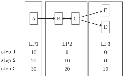
For an eﬃcient parallelization, we assume that the QPNs model can be decomposed into cycle-free partitions which can be described as Directed Acyclic Graph (DAG). This may sound like a strong restriction but can be accomplished throughout a smart decomposition for all performance mod-els with an open workload (i.e., the arrival rate is constant and independent of the processing of the system). We il-lustrate the idea using the example depicted in Figure 1. In this example, model elementsBandCare cyclically con-nected and have to be merged to receive a DAG. We name an LPApreceding to another LPBifAmay send tokens toB. ThenBis successor ofA. For an eﬃcient parallelization, each predecessor has to provide a good lookahead guarantee to its successor. In our approach, each LP passes itsclock value as

step 1

step 2

step 3

LP1 LP2 LP3

10 0 0

20 10 0

30 20 10

A B C

D E

Figure 1: Stepwise virtual time propagation

a lookahead border to its succeeding LPs. To enable parallel execution, it is necessary that LPs are ahead in time of pre-ceding LPs, which has to be ensured by the program logic. Figure 1 shows an example procedure. In the ﬁrst step only

LP1is processing ten time steps. In the next step, addition-allyLP2processes until reaching the lookahead border of 10 granted by LP1. Before entering the third step,LP1 grants lookahead border of 20 toLP2andLP2grants execution until 10 toLP3. Starting from the third step, all LPs may process ten time units per synchronization step. For every step, the lookahead of an LP can be set to the minimum time of its predecessor(s). Referring to the example, the key parts for our parallel simulation are:

Stepwise time propagation. Predecessors of LP have to

be ahead in time to enable parallel execution. To re-duce the synchronization overhead, we we propose a stepwise increment if no cycles exist. The time step size, which has been set to10in the example, can be tuned for a concrete scenario.

DAG decomposition. The requirement of a cycle-free

ini-tial model can be relaxed dramatically through smart decomposition. The initial model may contain cycles. The transformation to a DAG happens by merging all cycle elements into one LP. As a consequence, the model is free of cycles on the LP meta-level.

(5)

Our approaches for stepwise time propagation and DAG decomposition may be ported to formalisms other than QPNs

as well. The LPs A, B or C could stand for queues of a

QN or a set of places and transitions in a Stochastic Petri Net (SPN) or subparts of other formalisms.

4.2 Implementation

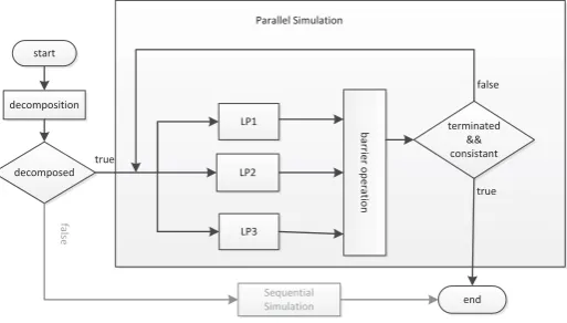
Our simulation process for the three LPs of the initial example is depicted in Figure 2. The newly implemented parallel simulation starts if the model can be decomposed to a DAG. Otherwise, sequential simulation is started auto-matically. Thereby, the user does not need to consider the the suitability of a model for parallel simulation. The

limita-LP1 _terminated && consistant LP2

decomposition

LP3

barrier operation

start

end

Sequential Simulation

decomposed

fal

se

true

true false Parallel Simulation

Figure 2: Parallel Simulation Process

tion to models that can be decomposed to a DAG inﬂuences the choice of parallelization techniques and paradigms. Op-timistic parallelization would result in additional overheads (e.g., for state saving) in order to increase intervals between synchronizations. The stepwise time concept enables to

in-crease these intervals to an arbitrary length. Hence, we

minimize computational overhead by applying conservative synchronization where the minimal clock of the predeces-sors of an LP is used as its lookahead. The next choice is on synchronous or asynchronous communication. We apply a synchronous barrier-based parallelization, as the global bar-rier operation enables efficient lookahead updates. During each barrier operation the simulation engine updates the lookahead time for each LP. Then each LP processes all events in its safe to process time range and enters the bar-rier afterwards. The procedure repeats until the stopping criterion of the simulation is fulfilled and and the model is in a consistent state again. During parallel simulation the LPs have different virtual times which results in a glob-ally inconsistent state of the model, as depicted in Figure 1. A consistent state is restored on simulation termination by choosing the event with the highest timestamp (which re-sides within an LP with no predecessors) and processing all events with smaller timestamps. Token generation at LPs without predecessors stops and then the LPs process all re-maining events up to the stopping virtual time. Finally, we equalize time so that all LPs have the same virtual time which results in a consistent global state again. During this consistency step, a few additional events may be simulated compared to sequential simulation. However, given that the

stopping criteria is speciﬁed as a minimum requirement on the accuracy, this does not invalidate the results.

The time safe to process for each LP is set during barrier operation. The mechanism depends on whether an LP has predecessors or not. In models with open workloads, at least one LP exists without predecessors exists (calledworkload generatorin the following). The absence of predecessors (i.e. no incoming events) implies the absence of lookahead con-straints. An infinite lookahead prohibits a balanced simula-tion as the LP would never enter the barrier. Consequently, we require an artificial lookahead border which forces the LP to enter the barrier. Ideally, this artificial border cre-ates a balanced token flow between LPs to get a balanced simulation. The decision for the artificial lookahead border size depends on the implementation and is a possible candi-date for auto-tuning mechanisms. If the border is chosen too small the workload-generator LP sends few or even no tokens to its successors. This results in multiple barrier operations with low progress. A long period allows for processing of multiple events which may result in a surge of events be-ing sent to the successor LPs. The incombe-ing token list of an LP is a priority queue and insertions get more expensive with increasing queue length. We refined the idea of a user defined time interval in the form of a specified number of tokens to be processed before entering the barrier. Thereby, a more constant token flow can be generated and a sensitive time step size parameter can be avoided.

Parallel simulation depicts a special case, where standard barrier implementations fail to achieve good performance. In standard barrier implementations, as e.g., provided by the Java standard library, threads leave the CPU while wait-ing on a barrier. Especially in Java, this wait step causes an expensive operating system operation [3]. Instead of expen-sive pasexpen-sive wait, active wait saves the costs for leaving and reentering CPU. In many application scenarios, the costs for barrier operations are negligible. In parallel simulation, we enter the barrier very frequently (every fewmicroseconds). Hence, active wait helps to reduce the synchronization over-heads signiﬁcantly. Another problem of standard implemen-tations is the access contention on the entering function of a barrier. This access contention can be parallelized using hierarchical barriers [3]. We employ the barrier implementa-tion of Peschlow et al. [35] for our parallel simulaimplementa-tion engine. Their implementation utilizes the described techniques for high frequency parallel simulation.

4.3 Decomposition

(6)

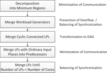
Fer-Decomposition into Minimum Regions

Merge Workload Generators

Merge Cyclic Connected LPs

Prevention of Overflow / Balancing of Synchronization

Minimization of Communication Minimization of Communication

Merge LPs with Ordinary Input Places into Predecessors

Balancing of Synchronization Merge LPs Until

Number of LPs < Number of Cores

Transformation to DAG

Figure 3: Decomposition Scheme

scha [10] to QPNs. A minimum region includes all places that share one transition and all transitions for which one of these places is an input place. The advantage of the mini-mum region idea is that the choice which transition fires next resides in one minimum region which reduces communica-tion overheads for parallel simulacommunica-tion. After decomposicommunica-tion in minimum regions, they can be assembled to larger units. We now describe our merging process for the minimum re-gions which results in a DAG which has only one LP without predecessors. An overview of the decomposition process is depicted in Figure 3. At first, we ensure constant token flow in case more than one workload generator exists. In that scenario, one workload generator may increase its vir-tual time faster than the others which may result in overflow situations. We prevent this by merging all workload genera-tors into one LP. Another option would be to artificially set one workload generator as predecessors for the other work-load generators. Next, we remove any cycles between LPs by merging all cyclically connected LPs. We receive a DAG by merging all strongly connected sets detected by Tarjan’s algorithm [43]. Through the previous two steps, we obtain a DAG with only one LP without predecessors. Next, we merge LPs having ordinary places as input places into their predecessors. Transitions of such LPs fire directly whenever a token arrives at their ordinary incoming place(s). Conse-quently, there is no virtual time delay to their predecessors which makes them a suitable candidate for merging. Finally, we merge LPs until the number of LP is less or equal to the number of processor cores. The merging algorithm starts from the element with no predecessors and merges its suc-cessors until a certain size is reached. Then the procedure repeats with one of the successors. A more formal view of this algorithm is depicted in Algorithm 1. It receives a set of LPs (lps) which is merged until the number of LPs sinks below theupperBound. This parameter can either be set by the user or is automatically set to the number of available processor cores. Lines 4 to 14 show the merging process for the first #core−1 LPs. In the last step all remaining LPs are merged into the current to ensure that the total number of LPs is less or equal to the upper bound. The function

hasAdequateSizein line 8 is used to decide whether to in-crease the size of the current LP or to select one of the suc-cessors as new initial merging spot. The decision is based on a ratio of the current LP’s computational eﬀort compared to the total eﬀort. Our actual implementation uses LP’s place count as indicator for this but further factors, e.g., number of branchings, internal recursion depth, queues and their queueing strategies, may be included. In general, the number of LPs has not necessarily to be less or equal to the

number of cores when multiple LPs are assigned to a thread. We decided against this option as computational overheads would increase.

Algorithm 1Final Merging Step

1: functionmergeFinal(lps, upperBound)

2: current←getLPWithoutPredecessor(lps);

3: reachable← ∅

4: numLPs←1

5: whilenumLPs<cores;do

6: reachable.append(current.getSuccessors());

7: while ¬reachable.isEmpty()do

8: successor←reachable.removeFirst();

9: if ¬hasAdequateSize(current)then

10: current←merge(current, successor);

11: else if numLPs<coresthen

12: current←successor;

13: numLPs = numLPs + 1

14: else

15: if ¬reachable.isEmpty()then

17: end if

18: break;

19: end if

20: end while

21: end while

22: while ¬reachable.isEmpty()do

23: successor←reachable.removeFirst();

24: current←merge(current, successor);

25: if ¬reachable.isEmpty()then

27: end if

28: end while

29: end function

5. CASE STUDIES

We conducted a series of case studies with open workload models to evaluate the speedup achieved through barrier-based parallel simulation. For each model, we compare the runtime of the parallel to the sequential case. Speedup is deﬁned as the runtime of parallel implementation divided by the runtime of the sequential one. The signiﬁcance level is determined using a two-sided Student’s t-test rejecting the hypothesis that the runtime of parallel and sequential executions belong to one set. A validation which shows that sequential and parallel simulation yield the same results with equal accuracy has been performed in [46].

(7)

Sec-tion 5.2 presents a medium-scale model of the SPECj Ap-plication Server benchmark. The case study presented in Section 5.3 uses a network model that has been generated by an automated transformation. Section 5.4 systematically evaluates diﬀerent aspects of our implementation using a synthetic model.

5.1 Layered Architecture Model of a Large

SaaS Provider

The QPN model shown in Figure 4 describes the perfor-mance behavior of a Customer Relation Ship (CRM) appli-cation of a large SaaS cloud provider in a simpliﬁed form. The model represents an application scenario comprising

AppServer1CPU1

OpenWorkload/4 tstart LoadBalancer tas1 tas1end tasend tdbDBServerCPU1 tend trash

Figure 4: Performance Model Decomposition

two application servers (in our case each with 6 cores), a load balancer, a database server and a delay incurred by the storage system. The model has nine token colors, rep-resenting nine diﬀerent transaction types. We measured the simulation runtime at QPME statistics level 4 (i.e., includ-ing response time histograms). The average speedup was 1.91 with signiﬁcance level of 7.70290e−9. This example shows that even for small models speedup is possible with our approach.

5.2 SPECjAppServer2004

The QPN model in Figure 5 describes a deployment of the SPECj Application Server benchmark. The model contains a load balancer, a replicated application server tier and a replicated database tier. The model is based on the case study presented in [23]. We changed the model to an open workload using an equivalent parametrization. The model

Figure 5: SPECj Application Server Benchmark

Modeled With Open Workload

of the load balancer (T,L, t3, t4) includes a circular struc-ture. To apply our stepwise virtual time all elements of a cycle have to be merged into one LP. Compared to the de-composition algorithm described in Section 4.3, we merged

OpenWorkload5intoEinstead of merging it with OpenWork-load6 to improve load balancing. We obtained an aver-age speedup of 2.45 using 4 cores with a signiﬁcance level of 2.04099e−18. In general, we expect increased speedups through better load balancing as the model size increases.

5.3 Network Trafﬁc Model

The network traﬃc model for this case study was gen-erated using the DNI-to-QPN transformation published in [37]. Compared to QNs, QPNs oﬀer advantages for modeling software contention in switches. The model has one server connected to another server by one switch. We applied a fully automated decomposition. We omit the depiction of the model due to space constraints.

Number of Threads/ LPs 2 3 4

Speedup 1.61 1.92 2.22

5.4 Synthetic Model

The previous subsections demonstrated the real-world ap-plicability of parallel QPN simulation. However, a synthetic model allows for a systematic investigation of the scalability and speedup potential of our implementation. This section shows that the main reason for deviation from linear speedup is a non-optimally balanced decomposition.

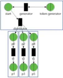
We used a synthetic model that generates tokens and dis-tributes them to multiple lanes. The structure for token generation and distribution remains constant whereas the number and length of lanes can be varied. Models are gen-erated asm×n. Variablemrepresents the number of lanes

andnis the number of queueing places. Figure 6 shows an

example of a 3×2 model.

Figure 6: Generated Model With Three Lanes, Each of Length Two Queueing Places.

The model is partitioned into the constant token gener-ation part and lanes, each representing an LP, so that the lanes execute in parallel. The two parametersmandnvary two aspects. The length of a lane determines the amount of operations between barrier synchronizations. The number of lanes determines the number LPs and thereby the num-ber of cores that can be utilized. The synthetic model allows to specify an upper bound for the theoretical speedup which enables a comparison with actual measured execution times.

speedup=m×f(m, n) +k (1)

(8)

upper bound for speedup as

speedup=m+ 1 (2)

The ﬁrst experiment we present keeps m = 6 ﬁxed and

varies the length of the lanen. Figure 7 shows speedups com-pared ton. As expected, an increasednincreases speedup.

0 4 8 12 16 20

0 20 40 60 80 100 120

sp

ee

d

up

length of lane

Figure 7: Speedup for Length of Lanes Variation

However, the experiments even show speedups above the theoretical optimum. This can be explained by two divide-and-conquer benefits of the parallel implementation. Firstly, we benefit formcache effects. Subproblems are smaller and can be kept in the cache. The parallel version is faster be-cause of cheaper cache accesses instead of “expensive” RAM accesses. The second divide and conquer effect is algorith-mic. The parallel version performs the choice of the next transition to fire LP-locally. Thereby less concurrently en-abled transitions occur compared to the global solution and unnecessary choices for the next transition can be omitted.

0 1 2 3

0 1 2 3 4 5 6 7

sp

eedup

number of lanes

Figure 8: Speedup for Lane Number Variation

The second experiment, depicted in Figure 8, varies the

number of lanes and keeps the length n = 2 ﬁxed. The

setup poses a very small load for the LPs, which reveals the barrier contention eﬀect. The speedup is proportional to the number of lanes up to an asymptotic border. After that the speedup may even decline. The reason is the global

barrier which becomes a bottleneck for high numbers of LPs. We optimized for common use cases at the expense of a scalability limitation. However, in scenarios where the load between barrier operations is higher, the asymptotic bound would appear at a much higher number of cores.

6. RELATED WORK

The question about suitability for parallel simulation has been answered for different types of models in different do-mains. To the best of our knowledge, no previous work con-sidered the potential of QPN models for speedup through parallel discrete-event simulation. The only previous work we are aware of that considers the concurrent simulation of QPNs was presented in a master’s thesis [18]. However, the thesis does neither consider any formalism specific as-pect like lookahead for queues nor does it consider model decomposition. Instead the thesis provides a performance test for well known conservative and optimistic scheduling algorithms. Our work is the first to consider formalism spe-cific discrete-event simulation of QPNs. The parallelization of a DAG, as we proposed, has been performed in different research areas. However, we could not find applications to simulation. The majority of related work is on paralleliza-tion on the event level for TPNs and QNs. Most publicaparalleliza-tions in this area propose different algorithms optimized for differ-ent model use cases. In the following, we presdiffer-ent a selection: A set of approaches build on specialized hardware, like vec-tor machines or Graphics Processing Units (GPUs), which have a Single Instruction Multiple Data (SIMD) architec-ture. This hardware is able to solve vector operations very fast that appear when solving PN recurrence equations. For vector machines, SPN analysis has been parallelized [2]. For GPUs, SPN [16] and Hybrid Functional Petri Nets (HFPNs) [9] analysis has been parallelized. All SIMD approaches have in common that speedup is reached by specialized hardware matrix operations on sparse matrices but not by an efficient strategy. Multiple LP-based discrete-event parallelizations for QNs and TPNs have been proposed. Nicol and Roy [31] apply a conservative synchronization protocol for discrete-event analysis of TPNs. They propose a tripartition discrete-event types to improve efficiency. Chiola and Ferscha [10] describe how TPNs can be split in LPs to apply conservative and

time warp synchronization. They deﬁne minimum regions

(9)

7. CONCLUSION

We investigated the feasibility for parallel discrete-event QPN simulation. The QPN formalism inherits bad looka-head characteristics from its subformalisms, which makes QPNs a challenging candidate for parallel simulation. How-ever, we showed that QPN models with open workloads are suitable for parallel execution. Support for parallel simula-tion of such models has been integrated into a general open-source simulation engine and extensively tested.

The experiments show speedups of 1.9 using 3 threads and 2.5 using 4 threads in the context of real-world case studies. In general, higher speedups are possible. The scal-ability analysis we presented using artiﬁcial models demon-strates that our implementation can provide up to super-linear speedups. During our work on parallel QPN simu-lation, many new questions arose. We consider improve-ments on decomposition to be the most promising ﬁeld for future work. We apply a decomposition to minimum re-gions and use a set of merging rules. The decomposition can be improved by the use of runtime statistics. Furthermore, our currently static partitioning does not consider changing workloads during simulation. For further research, we pro-pose a dynamic partitioning approach which could improve load balancing during a simulation run. Furthermore, addi-tional case studies with large scale models can be conducted to further evaluate the scalability of the parallel simulation approach.

8. REFERENCES

[1] H. Ammar and S. Deng. Time warp simulation of stochastic petri nets. InPetri Nets and Performance Models, 1991. PNPM91., Proceedings of the Fourth International Workshop on, pages 186–195, Dec 1991. [2] F. Baccelli and M. Canales. Parallel simulation of

stochastic petri nets using recurrence equations.ACM Transactions on Modeling and Computer Simulation, 3:20–41, 1993.

[3] C. Ball and M. Bull. Barrier synchronisation in java.

Available from World Wide Web: http://www. ukhec. ac. uk/publications/reports/synch java. pdf, 2003. [4] F. Bause. Queueing petri nets-a formalism for the

combined qualitative and quantitative analysis of

systems. InPetri Nets and Performance Models, 1993.

Proceedings., 5th International Workshop on, pages 14 –23, oct 1993.

[5] F. Bause, P. Buchholz, and P. Kemper. Qpn-tool for the speciﬁcation and analysis of hierarchically

combined queueing petri nets. InBAUSE (EDS.)

QUANTITATIVE EVALUATION OF COMPUTING AND COMMUNICATION SYSTEMS, LECTURE NOTES IN COMPUTER SCIENCE, pages 224–238. Springer, 1995.

[6] F. Bause and P. S. Kritzinger.Stochastic Petri nets -an introduction to the theory (2. ed.). Vieweg, 2002. [7] S. Becker, H. Koziolek, and R. Reussner. The Palladio

component model for model-driven performance prediction.Journal of Systems and Software, 82:3–22, 2009.

[8] F. Brosig, P. Meier, S. Becker, A. Koziolek,

H. Koziolek, and S. Kounev. Quantitative Evaluation of Model-Driven Performance Analysis and Simulation

of Component-based Architectures.IEEE

Transactions on Software Engineering (TSE), 2014. Accepted for publication.

[9] G. Chalkidis, M. Nagasaki, and S. Miyano. High performance hybrid functional petri net simulations of

biological pathway models on cuda.Computational

Biology and Bioinformatics, IEEE/ACM Transactions on, 8(6):1545–1556, Nov.-Dec. 2011.

[10] G. Chiola and A. Ferscha. Distributed simulation of timed petri nets: Exploiting the net structure to obtain eﬃciency. In M. Ajmone Marsan, editor,

Application and Theory of Petri Nets 1993, volume 691 ofLecture Notes in Computer Science, pages 146–165. Springer Berlin Heidelberg, 1993.

[11] X. Fang, Z. Xu, and Z. Yin. Distributed processing based on timed petri nets. InProceedings of the Third International Conference on Natural Computation -Volume 05, ICNC ’07, pages 287–291, Washington, DC, USA, 2007. IEEE Computer Society.

[12] A. Ferscha. Adaptive time warp simulation of timed petri nets.Software Engineering, IEEE Transactions on, 25(2):237–257, Mar/Apr 1999.

[13] R. M. Fujimoto. Lookahead in parallel discrete event simulation. Technical report, DTIC Document, 1988. [14] R. M. Fujimoto. Parallel and distributed discrete

event simulation: algorithms and applications. In

Proceedings of the 25th conference on Winter simulation, WSC ’93, pages 106–114, New York, NY, USA, 1993. ACM.

[15] R. M. Fujimoto.Parallel and Distribution Simulation Systems. John Wiley & Sons, Inc., New York, NY, USA, 1st edition, 2000.

[16] R. Geist, J. Hicks, M. Smotherman, and J. Westall. Parallel simulation of petri nets on desktop pc hardware. InSimulation Conference, 2005 Proceedings of the Winter, page 10 pp., dec. 2005.

[17] K. Jensen. Coloured Petri Nets and the

invariant-method.Theoretical Computer Science, 14:317–336, 1981.

[18] T. J¨urgens. Verteilte simulation von hqpns auf einem netzwerk von workstations. Master’s thesis,

Universit¨at Dortmund, Fachbereich Informatik, 1997. [19] F. J. Kaudel. A literature survey on distributed

discrete event simulation.SIGSIM Simul. Dig., 18(2):11–21, June 1987.

[20] D. G. Kendall. Stochastic processes occurring in the theory of queues and their analysis by the method of

the imbedded markov chain.The Annals of

Mathematical Statistics, 24(3):338–354, 1953. [21] S. Kounev.Performance Engineering of Distributed

Component-Based Systems - Benchmarking, Modeling and Performance Prediction. Shaker Verlag, Ph.D. Thesis, Technische Universit¨at Darmstadt, Germany, Aachen, Germany, December 2005. Best Dissertation Award from the ”Vereinigung von Freunden der Technischen Universit¨at zu Darmstadt e.V.”. [22] S. Kounev. Performance modeling and evaluation of

distributed component-based systems using queueing petri nets.Software Engineering, IEEE Transactions on, 32(7):486 –502, july 2006.

(10)

International Symposium on Performance Analysis of Systems and Software (ISPASS 2003), Austin, Texas, USA, March 6-8, 2003, pages 143–155, Washington, DC, USA, 2003. IEEE Computer Society.

Best-Paper-Award at ISPASS-2003.

[24] S. Kounev and A. Buchmann. SimQPN - a tool and methodology for analyzing queueing Petri net models by means of simulation.Performance Evaluation, 63(4-5):364–394, May 2006.

[25] S. Kounev and A. Buchmann. On the Use of Queueing Petri Nets for Modeling and Performance Analysis of Distributed Systems. In V. Kordic, editor,Petri Net, Theory and Application. Advanced Robotic Systems International, I-Tech Education and Publishing, Vienna, Austria, February 2007.

[26] S. Kounev and S. Spinner.QPME 2.0 User’s Guide,

2011.

[27] Y.-B. Lin and E. Lazowska. Exploiting lookahead in parallel simulation.Parallel and Distributed Systems, IEEE Transactions on, 1(4):457–469, 1990.

[28] P. Meier, S. Kounev, and H. Koziolek. Automated transformation of component-based software architecture models to queueing petri nets. In19th IEEE/ACM International Symposium on Modeling, Analysis and Simulation of Computer and

Telecommunication Systems (MASCOTS 2011), Singapore, July 25–27, 2011.

[29] P. Merkle. Comparing process- and event-oriented software performance simulation. Master’s thesis, Karlsruhe Institute of Technology (KIT), Germany, 2011.

[30] D. M. Nicol. Parallel discrete-event simulation of fcfs stochastic queueing networks. InProceedings of the ACM/SIGPLAN conference on Parallel programming: experience with applications, languages and systems, PPEALS ’88, pages 124–137, New York, NY, USA, 1988. ACM.

[31] D. M. Nicol and S. Roy. Parallel simulation of timed petri-nets. InProceedings of the 23rd conference on Winter simulation, WSC ’91, pages 574–583,

Washington, DC, USA, 1991. IEEE Computer Society. [32] P. O. Nierstrasz. Concurrent programming. Lecture,

1999.

[33] A. Nketsa and N. B. Khalifa. Timed petri nets and prediction to improve the chandy-misra

conservative-distributed simulation.Applied Mathematics and Computation, 120(1-3):235 – 254, 2001.<ce:title>The Bellman Continuum</ce:title>. [34] R. Osman, D. Coulden, and W. Knottenbelt.

Performance modelling of concurrency control schemes for relational databases. In A. Dudin and K. Turck, editors,Analytical and Stochastic Modeling Techniques and Applications, volume 7984 ofLecture Notes in Computer Science, pages 337–351. Springer Berlin Heidelberg, 2013.

[35] P. Peschlow, A. Voss, and P. Martini. Good news for parallel wireless network simulations. InProceedings of the 12th ACM international conference on Modeling, analysis and simulation of wireless and mobile systems, MSWiM ’09, pages 134–142, New York, NY, USA, 2009. ACM.

[36] D. A. Reed, A. D. Malony, and B. McCredie. Parallel

discrete event simulation using shared memory.IEEE

Trans. Softw. Eng., 14(4):541–553, Apr. 1988. [37] P. Rygielski and S. Kounev. Data Center Network

Throughput Analysis using Queueing Petri Nets. In

34th IEEE International Conference on Distributed Computing Systems Workshops (ICDCS 2014 Workshops). 4th International Workshop on Data Center Performance, (DCPerf 2014), pages 100–105, June 2014.

[38] K. Sachs, S. Kounev, and A. Buchmann. Performance modeling and analysis of message-oriented

event-driven systems.Journal of Software and Systems Modeling (SoSyM), pages 1–25, February 2012. [39] M. Saliminia. Multi-tenant performance models to

guarantee performance isolation. Master’s thesis, Karlsruhe Institute of Technology (KIT), 2013. [40] B. Schroeder and M. Harchol-Balter. Web servers

under overload: How scheduling can help.ACM

Trans. Internet Technol., 6(1):20–52, Feb. 2006. [41] B. Schroeder, A. Wierman, and M. Harchol-Balter.

Open versus closed: A cautionary tale. InNSDI, volume 6, pages 18–18, 2006.

[42] S. Spinner, S. Kounev, and P. Meier. Stochastic modeling and analysis using qpme: Queueing petri net modeling environment v2.0. In S. Haddad and L. Pomello, editors,Proceedings of the 33rd

International Conference on Application and Theory of Petri Nets and Concurrency (Petri Nets 2012),

volume 7347 ofLecture Notes in Computer Science

(LNCS), pages 388–397. Springer-Verlag, 6 2012. [43] R. Tarjan. Depth-ﬁrst search and linear graph

algorithms.SIAM Journal on Computing,

1(2):146–160, 1972.

[44] D. B. Wagner and E. D. Lazowska. Parallel simulation of queueing networks: limitations and potentials. In

Proceedings of the 1989 ACM SIGMETRICS international conference on Measurement and modeling of computer systems, SIGMETRICS ’89, pages 146–155, New York, NY, USA, 1989. ACM. [45] D. B. Wagner, E. D. Lazowska, and B. N. Bershad.

Techniques for eﬃcient shared-memory parallel simulation. Technical Report TR-88-04-05, Dept of Computer Science, Univ. of Washington, Seattle, WA 98195, Aug. 1988.

[46] J. Walter. Parallel Simulation of Queueing Petri Net Models. Master thesis, Karlsruhe Institute of Technology (KIT), Am Fasanengarten 5, 76131 Karlsruhe, Germany, October 2013.

[47] B. L. Worthington, G. R. Ganger, and Y. N. Patt. Scheduling algorithms for modern disk drives. In

SIGMETRICS, pages 241–252, 1994.

Parallel Simulation of Queueing Petri Nets