Fuzzy Inventory Model for Deteriorating Items
with Exponentially Decreasing Demand under
Fuzzified Cost and Partial Backlogging
Bhabani S. Mohanty
1, P.K. Tripathy
2P.G. Department of Statistics, Utkal University, Bhubaneswar, Odisha, India – 751004
Abstract
Due to technological advancement and business competition, the demand of electronic commodity and software products decreases with time. So in the present paper, we develop an inventory model for deteriorating items with constant deterioration and exponentially decreasing demand. Shortages are allowed in the model and are partially backlogged. This model also considers fuzzy based cost components (holding cost, shortage cost etc.) and deterioration. All related costs are assumed to be trapezoidal fuzzy numbers. Here signed distance and gradient mean integration method is used for defuzzification. We provide simple analytical tractable procedure for optimal inventory replenishment policy of the model and give numerical examples to illustrate the result. Sensitivity analysis of the major parameters with respect to the optimal solution is also carried out. This paper provides an interesting topic for further study, such that the joint influence from some of these parameters may be investigated to show the effects.
Keywords: Graded Mean Integration, Signed Distance Method, Partial Backlogging.
1. INTRODUCTION
In inventory management, many researchers have studied inventory models for deteriorating items such as medicines, electronic components, software products and fashion goods. In formulating inventory models, there are two facts of problem, one being the deterioration of items, the other being the variation in the demand rate. In 1915, the first inventory model was developed by F. Harris .Dave and Patel [1981] who derived a lot size model for constant deterioration of items with time proportional demand. Sachan [1984] allowed shortages in Dave and Patel [1981]’s model.
In certain situations uncertainties are due to fuzziness, and such cases are dilated in the fuzzy set theory which was demonstrated by Zadehin[1965]. Kaufmann and Gupta[1991] provided an introduction to fuzzy arithmetic operation and Zimmermann[1985] discussed the concept of the fuzzy set theory and its
applications. Park [1987] applied the fuzzy set concepts to EOQ formula by representing the inventory carrying cost with a fuzzy number and solved the economic order quantity model using fuzzy number operations based on the extension principle. Vujosevic et al.[1996] used trapezoidal fuzzy number to fuzzify the order cost in the total cost of the inventory model without backorder, and got fuzzy total cost. Yao and Lee [1996] introduced a backorder inventory model with fuzzy order quantity as triangular and trapezoidal fuzzy numbers and shortage cost as a crisp parameter. Gen et al.[1997] expressed their input data as fuzzy numbers, and then the interval mean value concept was introduced to solve the inventory problem.In 2007, J. K. Syed and L. A. Aziz [2005] applied signed distance method to Fuzzy inventory model without shortages. P. K. Tripathy et al.[2008] developed an entropic order quantity model with fuzzy holding cost and fuzzy disposal cost for perishable items. In 2011, P. K. De and A. Rawat proposed a fuzzy inventory model without shortages using triangular fuzzy number. In 2012, C. K. Jaggi, S. Pareek, A. Sharma and Nidhi presented a fuzzy inventory model for deteriorating items with time-varying demand and shortages. In 2012, SumanaSaha and TriptiChakrabarti proposed a fuzzy EOQ model for time dependent deteriorating items and time dependent demand with shortages. Very recently, D. Dutta and Pavan Kumar published several papers in the area of fuzzy inventory with or with shortages. In 2012, D. Datt et al. presented a fuzzy inventory model without shortage using trapezoidal fuzzy number with sensitivity analysis. Narendra et al.[2016] proposed fuzzy inventory model with exponential demand and time-varying deterioration.
mean integration method. The solution for minimizing the fuzzy cost function has been derived.
2. Basic concept
A fuzzy set
A
~
on the given universal setX
is a set of order pairsA
~
(
x
,
A(
x
)
)
:
x
X
Where ~
:
X
[
0
,
1
]
A
is called membership function.The
-cut ofA
~
is defined by
:
(
)
,
0
x
x
A
AIf
R
is a real line, then a fuzzy number is a fuzzy setA
~
with membership function ~:
X
[
0
,
1
]
A
, havingthe following properties
(i)
A
~
is normal i.e. there existx
R
such that1
)
(
x
A
(ii)
A
~
is piecewise continuous.(iii)
sup
p
(
A
~
)
cl
x
R
:
A(
x
)
0
, wherecl
represents the closure of a set. (iv)
A
~
is a convex fuzzy set.3. Assumptions and Notation
This inventory model is developed on the basis of the following assumptions and notation:
a)
(
t
)
is the constant rate of deterioration where0
1
.
b)
D
(
t
)
ae
btwhere
a
,
b
0
is exponentially decreasing demand.c) Shortage is allowed and partially backlogged. d)
l
is the shortage cost per unit per unit time. e)
is the backlogging rate;0
1
.
f) Replenishment is instantaneous; lead time is zero. g)
T
is the length of the cycle.h)
A
is the order quantity.i)
h
is the holding cost per unit time. j)C
is the unit cost of an item. k)S
is the lost sale cost per unit.l)
TC
(
t
1,
T
)
is the total inventory cost per unit time. m)D
~
is the fuzzy demand.n)
C
~
is the fuzzy unit cost of an item.p)
h
~
is the fuzzy holding cost per unit per unit time. q)~
l
is the fuzzy shortage cost per unit time. r)S
~
is the fuzzy lost sale cost per unit. s)(
1,
)
~
T
t
TC
is the total fuzzy inventory cost per unit time.t)
TC
G(
t
1,
T
)
is the defuzzify value of(
1,
)
~T
t
TC
by applying Graded Mean Integration.
u)
TC
S(
t
1,
T
)
is the defuzzify value of(
1,
)
~T
t
TC
by applying Signed Distance Method.
4. Mathematical Model 4.1 Crisp Model
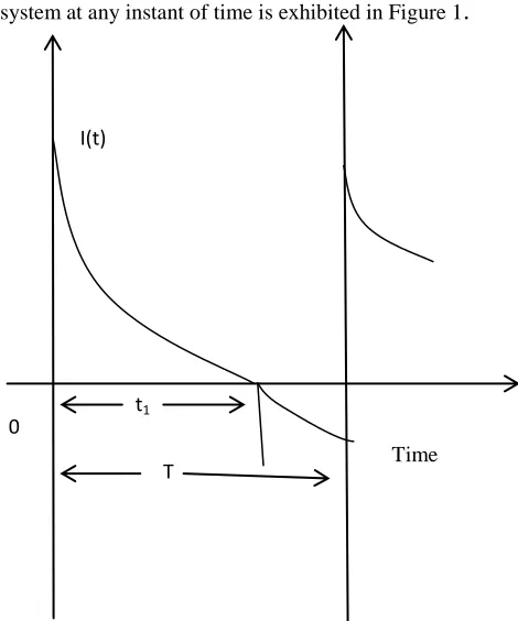
Under above assumption, the behaviour of inventory system at any instant of time is exhibited in Figure 1
.
Replenishment is made at time t=0 and the inventory level falls during the period [0, t1]. The inventory level is zero at t1. So shortages are allowed during the time interval [t1,T] and demand during this period is partially
Time
T
0 t1
I(t)
The rate of change of the inventory during the
positive stock period
(
0
,
t
1)
and shortage period)
(
t
1,T
is represented by the following differentialequations:
1 1
) (
0
),
(
)
(
)
(
1
t
I
t
D
t
t
t
dt t
dI
(1)
T
t
t
t
D
dt t
dI
1 )
(
),
(
1 (2)
The initial inventory level is
I
0 unit at time0
t
; fromt
0
tot
t
1, at this time, shortage isaccumulated which is partially backlogged at the rate β. Thus, boundary conditions are as follows:
0 1
(
0
)
I
I
,I
1(
t
1)
0
,I
2(
t
1)
0
. The solutions of equation (1) and (2) with boundary conditions are as follows1 )
(
1
(
)
,
0
1
t
t
dt
e
ae
t
I
t
t t b
t
(3)
2
1 2 2 1
2
(
t
)
a
T
t
T
t
I
b
(4)Using equation (3), we get the following
dt
e
a
I
I
t t b
10 ) ( 0
1
(
0
)
(5)
Inventory is available in the system during the
time interval
(
0
,
t
1)
. Hence, the cost for holdinginventory in stock is computed for time period
(
0
,
t
1)
only.
Holding cost is as follows:
dt
t
I
t
h
HC
t
10
1
(
)
)
(
4
1 8 3 1 3 3 1 6 2 1 2
1
t
t
t
t
ah
HC
b
b (6)Shortage due to stock out is accumulated in the
system during the interval
(
t
1,T
)
.The optimum levelof shortage is present at
t
T
; therefore, the totalshortage cost during this time period is as follows
T
t
dt
t
I
l
SC
1
)
(
2
)
(
)
(
)
(
2 12 1 2 11
abl
T
t
T
t
t
T
al
(7)Due to stock out during
(
t
1,T
)
, shortage isaccumulated but not all customers are willing to wait for the next lot size to arrive. Hence, this results in some loss of sale which accounts to loss in profit.Lost sale cost is calculated as follows:
T
t
dt
t
D
S
LSC
1)
(
)
1
(
)
(
)
(
)[
1
(
a
T
t
1 2T
2t
12S
ab
(8)Purchase cost is as follows:
)
)
(
(
1 0
T
t
dt
t
D
I
C
PC
)
(
)
(
)
(
21 2 121 2
1 2
1
t
aC
T
t
abC
T
t
t
Ca
b
(9)
Thus, total cost is as follows:
LSC
SC
HC
PC
OC
T
t
TC
(
1,
)
)]
(
)
(
[
)
1
(
)
(
)
(
)
(
)
(
)
(
)
(
)
,
(
2 1 2 2 1
1 2 1 2
1 2 1
4 1 8 3 1 6
2 2 1 2 1 2
1 2
2 1 1 2
1 2 1
1
t
T
t
T
a
S
t
T
t
T
abl
t
T
al
t
t
t
ah
t
T
abC
t
T
aC
t
t
Ca
A
T
t
TC
ab
b b b
(10)
To minimize the total cost
TC
(
t
1,
T
)
per unit time, the optimal value of T and t1 can be obtained by solving the following equations0
1
t
TC
and
0
T
TC
(11)
0
)
1
)(
1
(
)
(
)
(
2
)
]
)
(
1
[
1 2 1 2 1 1 3 1 2 2 1 2 2 1 1 1
bt
Sa
t
T
abl
t
T
al
t
t
t
ah
abCt
aC
t
b
Ca
b b
(12)0
)
1
)(
1
(
)
(
)
(
2
23 1 21
bT
Sa
t
T
abl
t
T
al
abCT
aC
(13)4.2 Fuzzy Model
Let
)
,
,
,
(
~
),
,
,
,
(
~
),
,
,
,
(
~
),
,
,
,
(
~
4 3 2 1 4 3 2 1 4 3 2 1 4 3 2 1C
C
C
C
C
h
h
h
h
h
b
b
b
b
b
a
a
a
a
a
)
,
,
,
(
~
),
,
,
,
(
~
4 3 2 1 4 3 21
l
l
l
S
S
S
S
S
l
l
aretrapezoidal fuzzy number.
Total cost of the system in fuzzy sense is given by
)]
(
)
(
~
)[
1
(
~
)
(
)
(
~
~
~
)
(
~
~
~
~
)
(
~
~
~
)
(
~
~
)
(
~
~
)
,
(
2 1 2 2 ~ ~ 1 1 2 1 2 1 2 1 4 1 8 ~ ~ 3 1 6 ~ 2 ~ 2 1 2 1 2 1 2 2 1 1 2 1 2 ~ ~ 1 1 ~t
T
t
T
a
S
t
T
t
T
l
b
a
t
T
l
a
t
t
t
h
a
t
T
C
b
a
t
T
C
a
t
t
a
C
A
T
t
TC
b a b b b
(14)(i) By Graded Mean Integration, total cost is given by
)
,
(
)
,
(
2
)
,
(
2
)
,
(
6
1
)
,
(
1 1 1 1 1 4 3 2 1T
t
TC
T
t
TC
T
t
TC
T
t
TC
T
t
TC
G G G G G (15) Where
)]
(
)
(
)[
1
(
)
(
)
(
)
(
)
(
)
(
)
(
)
,
(
2 1 2 2 1 1 1 1 2 1 1 1 1 2 1 2 1 1 1 4 1 8 3 1 6 2 2 1 2 1 1 1 2 1 2 1 1 1 2 1 1 1 1 2 1 2 1 1 1 1 1 1 1 1 1 1 1 1 1t
T
t
T
a
S
t
T
t
T
l
b
a
t
T
l
a
t
t
t
h
a
t
T
C
b
a
t
T
C
a
t
t
a
C
A
T
t
TC
b a b b b G
)]
(
)
(
)[
1
(
)
(
)
(
)
(
)
(
)
(
)
(
)
,
(
2 1 2 2 1 2 2 1 2 1 2 2 2 2 1 2 1 2 2 4 1 8 3 1 6 2 2 1 2 1 2 2 2 1 2 2 2 2 2 1 1 2 2 2 1 2 1 2 2 1 2 2 2 2 2 2 2 2 2t
T
t
T
a
S
t
T
t
T
l
b
a
t
T
l
a
t
t
t
h
a
t
T
C
b
a
t
T
C
a
t
t
a
C
A
T
t
TC
b a b b b G
)]
(
)
(
)[
1
(
)
(
)
(
)
(
)
(
)
(
)
(
)
,
(
2 1 2 2 1 3 3 1 2 1 3 3 3 2 1 2 1 3 3 4 1 8 3 1 6 2 2 1 2 1 3 3 2 1 2 3 3 3 2 1 1 3 3 2 1 2 1 3 3 1 3 3 3 3 3 3 3 3 3t
T
t
T
a
S
t
T
t
T
l
b
a
t
T
l
a
t
t
t
h
a
t
T
C
b
a
t
T
C
a
t
t
a
C
A
T
t
TC
b a b b b G
)]
(
)
(
)[
1
(
)
(
)
(
)
(
)
(
)
(
)
(
)
,
(
2 1 2 2 1 4 4 1 2 1 4 4 4 2 1 2 1 4 4 4 1 8 3 1 6 2 2 1 2 1 4 4 2 1 2 4 4 4 2 1 1 4 4 2 1 2 1 4 4 1 4 4 4 4 4 4 4 4 4t
T
t
T
a
S
t
T
t
T
l
b
a
t
T
l
a
t
t
t
h
a
t
T
C
b
a
t
T
C
a
t
t
a
C
A
T
t
TC
b a b b b G
To minimize total cost function per unit time
)
,
(
t
1T
TC
G the optimal value oft
1andT
can be obtained by solving the following equations0
)
,
(
1 1
t
T
t
TC
Gand
(
1,
)
0
T
T
t
TC
G (16)
0
)
1
)(
1
(
)
(
)
(
2
]
)
(
1
[
)
1
)(
1
(
)
(
)
(
2
]
)
(
1
[
2
)
1
)(
1
(
)
(
)
(
2
]
)
(
1
[
2
)
1
)(
1
(
)
(
)
(
2
]
)
(
1
[
6
1
1 4 4 4 2 1 4 4 4 2 1 1 4 4 3 1 2 2 1 2 2 1 4 4 1 4 4 4 4 4 1 4 4 4 4 1 3 3 3 2 1 3 3 3 2 1 1 3 3 3 1 2 2 1 2 2 1 3 3 1 3 3 3 3 3 1 3 3 3 3 1 2 2 2 2 1 2 2 2 2 1 1 2 2 3 1 2 2 1 2 2 1 2 2 1 2 2 2 2 2 1 2 2 2 2 1 1 1 1 2 1 1 1 1 2 1 1 1 1 3 1 2 2 1 2 2 1 1 1 1 1 1 1 1 1 1 1 1 1 1 4 4 4 4 3 3 3 3 2 2 2 2 1 1 1 1
t
b
a
S
t
T
l
b
a
t
T
l
a
t
t
t
h
a
t
C
b
a
C
a
t
b
a
C
t
b
a
S
t
T
l
b
a
t
T
l
a
t
t
t
h
a
t
C
b
a
C
a
t
b
a
C
t
b
a
S
t
T
l
b
a
t
T
l
a
t
t
t
h
a
t
C
b
a
C
a
t
b
a
C
t
b
a
S
t
T
l
b
a
t
T
l
a
t
t
t
h
a
t
C
b
a
C
a
t
b
a
C
b b b b b b b b
(17) And0
)
1
)(
1
(
)
(
)
(
2
)
1
)(
1
(
)
(
)
(
2
2
)
1
)(
1
(
)
(
)
(
2
2
)
1
)(
1
(
)
(
)
(
2
6
1
4 4 4 2 1 4 4 4 2 3 1 4 4 4 4 4 4 4 3 3 3 2 1 3 3 3 2 3 1 3 3 3 3 3 3 3 2 2 2 2 1 2 2 2 2 3 1 2 2 2 2 2 2 2 1 1 1 2 1 1 1 1 2 3 1 1 1 1 1 1 1 1
T
b
a
S
t
T
l
b
a
t
T
l
a
T
C
b
a
C
a
T
b
a
S
t
T
l
b
a
t
T
l
a
T
C
b
a
C
a
T
b
a
S
t
T
l
b
a
t
T
l
a
T
C
b
a
C
a
T
b
a
S
t
T
l
b
a
t
T
l
a
T
C
b
a
C
a
(18)(ii) By Signed Distance Method, total cost is
)
,
(
)
,
(
)
,
(
)
,
(
4
1
)
,
(
1 1 1 1 1 4 3 2 1T
t
TC
T
t
TC
T
t
TC
T
t
TC
T
t
TC
S S S S S (19) Where
)
(
)
(
)[
1
(
)
(
)
(
)
(
)
(
)
(
)
(
)
,
(
2 1 2 2 1 1 1 1 2 1 1 1 1 2 1 2 1 1 1 4 1 8 3 1 3 3 1 6 2 1 2 1 1 1 2 1 2 1 1 1 2 1 1 1 1 2 1 2 1 1 1 1 1 1 1 1 1 1 1 1 1t
T
t
T
a
S
t
T
t
T
l
b
a
t
T
l
a
t
t
t
t
h
a
t
T
C
b
a
t
T
C
a
t
t
a
C
A
T
t
TC
b a b b b S
)
(
)
(
)[
1
(
)
(
)
(
)
(
)
(
)
(
)
(
)
,
(
2 1 2 2 1 2 2 1 2 1 2 2 2 2 1 2 1 2 2 4 1 8 3 1 3 3 1 6 2 1 2 1 2 2 2 1 2 2 2 2 2 1 1 2 2 2 1 2 1 2 2 1 2 2 2 2 2 2 2 2 2t
T
t
T
a
S
t
T
t
T
l
b
a
t
T
l
a
t
t
t
t
h
a
t
T
C
b
a
t
T
C
a
t
t
a
C
A
T
t
TC
b a b b b S
)
(
)
(
[
)
1
(
)
(
)
(
)
(
)
(
)
(
)
(
)
,
(
2 1 2 2 1 3 3 1 2 1 3 3 3 2 1 2 1 3 3 4 1 8 3 1 3 3 1 6 2 1 2 1 3 3 2 1 2 3 3 3 2 1 1 3 3 2 1 2 1 3 3 1 3 3 3 3 3 3 3 3 3t
T
t
T
a
S
t
T
t
T
l
b
a
t
T
l
a
t
t
t
t
h
a
t
T
C
b
a
t
T
C
a
t
t
a
C
A
T
t
TC
b a b b b S
)
(
)
(
)[
1
(
)
(
)
(
)
(
)
(
)
(
)
(
)
,
(
2 1 2 2 1 4 4 1 2 1 4 4 4 2 1 2 1 4 4 4 1 8 3 1 3 3 1 6 2 1 2 1 4 4 2 1 2 4 4 4 2 1 1 4 4 2 1 2 1 4 4 1 4 4 4 4 4 4 4 4 4t
T
t
T
a
S
t
T
t
T
l
b
a
t
T
l
a
t
t
t
t
h
a
t
T
C
b
a
t
T
C
a
t
t
a
C
A
T
t
TC
b a b b b S
To minimize total cost function per unit time
)
,
(
t
1T
TC
S the optimal value oft
1andT
can be obtained by solving the following equations0
)
,
(
1 1
t
T
t
TC
Sand
(
1,
)
0
T
T
t
TC
S (20)
0
)
1
)(
1
(
)
(
)
(
2
]
)
(
1
[
)
1
)(
1
(
)
(
)
(
2
]
)
(
1
[
)
1
)(
1
(
)
(
)
(
2
]
)
(
1
[
)
1
(
)
1
(
)
(
)
(
2
]
)
(
1
[
4
1
1 4 4 4 2 1 4 4 4 2 1 1 4 4 3 1 2 2 1 2 2 1 4 4 1 4 4 4 4 4 1 4 4 4 4 1 3 3 3 2 1 3 3 3 2 1 1 3 3 3 1 2 2 1 2 2 1 3 3 1 3 3 3 3 3 1 3 3 3 3 1 2 2 2 2 1 2 2 2 2 1 1 2 2 3 1 2 2 1 2 2 1 2 2 1 2 2 2 2 2 1 2 2 2 2 1 1 1 1 2 1 1 1 1 2 1 1 1 1 3 1 2 2 1 2 2 1 1 1 1 1 1 1 1 1 1 1 1 1 1 4 4 4 4 3 3 3 3 2 2 2 2 1 1 1 1
t
b
a
S
t
T
l
b
a
t
T
l
a
t
t
t
h
a
t
C
b
a
C
a
t
b
a
C
t
b
a
S
t
T
l
b
a
t
T
l
a
t
t
t
h
a
t
C
b
a
C
a
t
b
a
C
t
b
a
S
t
T
l
b
a
t
T
l
a
t
t
t
h
a
t
C
b
a
C
a
t
b
a
C
t
b
a
S
t
T
l
b
a
t
T
l
a
t
t
t
h
a
t
C
b
a
C
a
t
b
a
C
b b b b b b b b
(21) And0
)
1
)(
1
(
)
(
)
(
2
)
1
)(
1
(
)
(
)
(
2
)
1
)(
1
(
)
(
)
(
2
)
1
)(
1
(
)
(
)
(
2
4
1
4 4 4 2 1 4 4 4 2 3 1 4 4 4 4 4 4 4 3 3 3 2 1 3 3 3 2 3 1 3 3 3 3 3 3 3 2 2 2 2 1 2 2 2 2 3 1 2 2 2 2 2 2 2 1 1 1 2 1 1 1 1 2 3 1 1 1 1 1 1 1 1
T
b
a
S
t
T
l
b
a
t
T
l
a
T
C
b
a
C
a
T
b
a
S
t
T
l
b
a
t
T
l
a
T
C
b
a
C
a
T
b
a
S
t
T
l
b
a
t
T
l
a
T
C
b
a
C
a
T
b
a
S
t
T
l
b
a
t
T
l
a
T
C
b
a
C
a
(22)5. Numerical Example
Consider an inventory system with following parametric values.
The following numerical values of the parameter in proper unit were considered as input for numerical analysis of the model.
A
2000,C
10,a
200,b
2,
0.4,h
0.2,
0.8,l
4,S
6. The output of the model by using Mathematica 5.1 mathematical software is283038
.
0
1
t
,T
0
.
556074
and TC=2525.35.2 Fuzzy Model
If
A
=2000,a
~
(
185
,
195
,
205
,
215
)
,)
4
,
3
,
2
,
1
(
~
b
,C
~
(
7
,
9
,
11
,
13
)
,
0
.
8
,)
4
.
0
,
3
.
0
,
2
.
0
,
1
.
0
(
~
,)
28
.
0
,
22
.
0
,
16
.
0
,
1
.
0
(
~
h
,~
l
(
1
,
3
,
5
,
7
)
,)
5
.
9
,
8
,
5
.
6
,
5
(
~
S
by using Mathematica 5.1 mathematical software we get by Graded Mean Integration Method ist
1
0
.
241301
,391626
.
0
T
andTC
GD=2383.43 and by Signed Distance Method ist
1
0
.
229905
,T
0
.
379559
andTC
SD=2372.56.6.Sensitive Analysis
Table-1 (Graded Mean Integration Method) Parameter % of
Change
𝑡1 T
GD
TC
C
~
+50+25 -25 -50 0.071109 0.175812 0.288627 0.325126 0.383132 0.389681 0.391838 0.390934 2539.28 2465.92 2293.97 2199.56
a
~
+50+25 -25 -50 0.241301 0.241301 0.241301 0.241301 0.391626 0.391626 0.391626 0.391626 2575.14 2479.29 2287.57 2191.71
b
~
+50+25 -25 -50 0.144639 0.183454 0.339015 0.543457 0.256055 0.30966 0.532525 0.831165 2250.68 2303.28 2520.46 2807.75
~
+50-25 -50
0.241951 0.242597
0.391568 0.39151
2383.37 2383.3
l
~
+50+25 -25 -50
0.293314 0.27206 0.193209 0.109431
0.396487 0.39449 0.387233 0.379933
2391.02 2387.77 2377.48 2369.36
S
~
+50 +25-25 -50
0.267944 0.265436 0.219841 0.185391
0.386886 0.390109 0.394372 0.396905
2389.96 2388.27 2378.14 2369.95 A three dimensional graph is shown
Figure 2: Total average cost (Graded Mean Integration method) vs. t1 and T
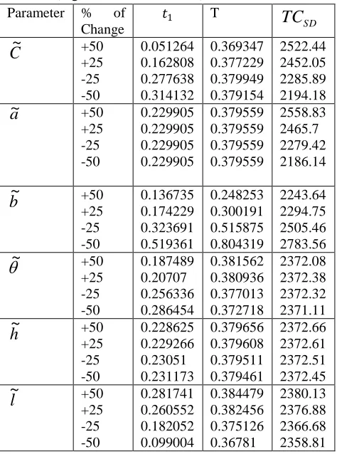
Table-2 (Signed Distance Method) Parameter % of
Change
𝑡1 T
SD
TC
C
~
+50 +25-25 -50
0.051264 0.162808 0.277638 0.314132
0.369347 0.377229 0.379949 0.379154
2522.44 2452.05 2285.89 2194.18
a
~
+50+25 -25 -50
0.229905 0.229905 0.229905 0.229905
0.379559 0.379559 0.379559 0.379559
2558.83 2465.7 2279.42 2186.14
b
~
+50 +25-25 -50
0.136735 0.174229 0.323691 0.519361
0.248253 0.300191 0.515875 0.804319
2243.64 2294.75 2505.46 2783.56
~
+50+25 -25 -50
0.187489 0.20707 0.256336 0.286454
0.381562 0.380936 0.377013 0.372718
2372.08 2372.38 2372.32 2371.11
h
~
+50+25 -25 -50
0.228625 0.229266 0.23051 0.231173
0.379656 0.379608 0.379511 0.379461
2372.66 2372.61 2372.51 2372.45
l
~
+50+25 -25 -50
0.281741 0.260552 0.182052 0.099004
0.384479 0.382456 0.375126 0.36781
2380.13 2376.88 2366.68 2358.81
S
~
+50 +25-25 -50
0.257594 0.245744 0.207055 0.168957
0.375128 0.377221 0.382023 0.383936
2379.33 2376.45 2366.97 2358.1
Figure 3: Total average cost (Signed Distance Method) vs. t1 and T
Based on results presented in Table 1, the following features are observed
o Total cost for Graded Mean Integration
increases rapidly with increase in the value of the model parameter
C
~
,a
~
,l
~
,S
~
.o Total fuzzy cost
TC
GD decreases with increase ofb
~
o There are negligence changes in fuzzy total cost
TC
GD when model parameters
~
andh
~
increasesFrom Table 2, the following observations can be made
o When
C
~
,a
~
,l
~
,S
~
increases thenTC
SD increases rapidlyo Total fuzzy cost for signed distance method (
SD
TC
) decreases with increase in value ofb
~
and almost insensitive for changes in
~
,h
~
.7. Conclusion and Analysis 0.1
0.2
0.3
0.4 t1
0.2 0.3
0.4 0.5
T 2300
2350 2400 KG
t1,T
0.1
0.2
0.3
0.4 t1
0.1 0.2
0.3
0.4 t1
0.2 0.3
0.4 0.5 T 2300
2325 2350 2375 2400
KS
t1,T
0.1 0.2
0.3
This paper represents a fuzzy inventory model for deteriorating items with allowable shortages in which demand is a decreasing exponential function. The demand, deterioration rate, inventory holding cost, shortage cost and lost sale cost are represented by trapezoidal fuzzy numbers. For defuzzificationgraded mean representation and signed distance method are employed to evaluate the optimal time period of positive stock
t
1and total cycle lengthT
which minimizes the total cost. By given numerical example it has been tested that signed distance method gives minimum cost as compared to graded mean representation.The proposed crisp model can be enriched by taking stochastic fluctuating demand patterns. In further, the fuzzy model can be changed by considering other type of membership functions such as piecewise linear hyperbolic and pentagonal fuzzy number.
Acknowledgements
The authors would like to thank Editorial Support Team and an anonymous referee for their constructive and positive comments and suggestions.
REFERENCES
1) De, P. K., & Rawat, A. (2011). A fuzzy inventory model without shortages using triangular fuzzy number. Fuzzy
Information & Engineering, 1, 59-68.
2) Dutta, D., & Kumar, P. (2012). Fuzzy inventory without shortages using trapezoidal fuzzy number with sensitivity analysis. IOSR Journal of mathematics, 4(3), 32-37. 3) Jaggi, C. K., Pareek, S., Sharma, A., & Nidhi. (2012). Fuzzy
inventory model for deteriorating items with time-varying demand and shortages. American Journal of Operational
Research, 2(6), 81-92.
4) Kaufman, A., & Gupta, M. (1991). Introduction to Fuzzy
Arithmatic. Van Nostrand Reinhold Company.
5) Sahoo, N. K., Mohanty, B. S., & Tripathy, P. K. (2016). Fuzzy inventory model with exponential demand and time-varying deterioration. Global Journal of Pure and Applied
Mathematics, 12(3), 2573-2589.
6) Syed, J. K., & Aziz, L. A. (2007). Fuzzy inventory model without shortages using signed. Applied Mathematics &
Information Sciences, 1(2), 203-209.
7) Tripathy, P. K., & Pattnaik, M. (2008). An entropic order quantity model with fuzzy holding cost and fuzzy disposal cost for perishable items under two component demand and discounted selling price. Pakistan Journal of Statistics and
Operation Research, 4(2), 93-110.
8) Tripathy, P. K., & Pattnaik, M. (2011). A fuzzy arithmetic approach for perishable items in discounted entropic order quantity model. International Journal of Scientific and
Statistical Computing, 1(2), 7-19.
9) Yao, J. S., & Lee, H. M. (1996). Fuzzy inventory with backorder for fuzzy order quanty. Information Sciences, 93, 283-319.
10) Zadeh, L. A. (1965). Fuzzy Sets. Information and Control, 8(3), 338-353.
11) Zimmermann, H. J. (1985). Application of fuzzy set theory to mathematical programming, Information Science.