A Population Based ACO Algorithm for the Combined Tours TSP Problem

(1)

A Population Based ACO Algorithm for the Combined

Tours TSP Problem

Martin Clauß

Fraunhofer FKIE Fraunhoferstraße 20

D-53343

Wachtberg-Werthhoven, Germany

Lydia Lotzmann

University of Leipzig Dept. of Computer Science

Augustusplatz 10 D-04109 Leipzig, Germany

Martin Middendorf

University of Leipzig Dept. of Computer Science

Augustusplatz 10 D-04109 Leipzig, Germany

ABSTRACT

In this paper we apply a Population based Ant Colony Op-timization (PACO) algorithm for solving the following new version of the Traveling Salesperson problem that is called the Combined Tours TSP (CT-TSP). Given are a set of cities, for each pair of cities a cost function and an integer

k. The aim is to ﬁnd a set ofk(cyclic) tours, i.e., each city

is contained exactly once in each tour and each tour returns to its origin city, which have minimum total costs. In this paper the case of finding two tours is studied where the costs of one tour depends on the other tour. Each pair of cities has a distance and a weight which influence the costs of the tours. The weight is used to define if it is advantageous or disadvantageous when the corresponding pair of cities is con-tained, i.e., neighbouring, in both tours. Different heuristics that the ants of the PACO use for the construction of the tours are compared experimentally. One result is that it is (often) advantageous when the heuristic for the second tour is different from the heuristic for the first tour such that the former heuristic uses knowledge about the first tour.

Categories and Subject Descriptors

I.2.8 [Artiﬁcial Intelligence]: Problem Solving, Control

Methods, and Search—Heuristic methods

Keywords

Ant colony optimization, population based ACO, traveling salesperson problem, metaheuristic

1. INTRODUCTION

A variant of the Traveling Salesperson problem is intro-duced in this paper where the aim is to ﬁnd for a given set of cities several (cyclic) tours such that each of them connects all given cities, i.e., each tour contains each city exactly once and returns to its origin city. The diﬃculty is that the costs

.

of each tour depend on the other tours and the total costs of all tours should be minimized. In the classical Travel-ing Salesperson problem (TSP) the aim is to ﬁnd a sTravel-ingle shortest, i.e., cheapest, (cyclic) tour. The TSP is one of the most investigated combinatorial optimization problems. It is an NP-hard problem and one of the standard benchmark problems that are used for testing metaheuristics. Many variants of the TSP have been studied in the literature (for an overview see Section 2).

In this paper we use the Population based Ant Colony Optimization metaheuristic (PACO) that was proposed in [7] to solve the new variant of the TSP. This variant is called Combined Tours TSP (TSP). An instance of the CT-TSP consists of a set of cities, for each pair of cities a cost

function (distance function), and an integer k ≥ 1. The

aim of the CT-TSP is to ﬁnd k (cyclic) tours which have

minimum total costs. The cost function for a pair of cities

(i, j) assigns for each tour that includes a drive from i to

j a corresponding cost. We are interested in particular in

cost functions where the costs that a tour has for driving

fromitojdepend on how many other tours include a drive

from i to j. The notation k-TSP is used for the

CT-TSP with ﬁxedk. In this initial study on the CT-TSP we

restrict us to the 2-CT-TSP, i.e., to the case of ﬁndingk= 2

tours. Note, that 1-CT-TSP is the standard TSP problem. Observe, that the special case where it holds for every pair

of cities (i, j) that the cost for driving fromitojis always

the same ﬁxed value dij can be reduced to the standard

TSP problem. Simply, choosingk times the cheapest TSP

tour is the optimal solution. It follows thatk-CT-TSP is an

NP-hard problem for everyk≥1.

As an application of the CT-TSP consider a scenario where companies have to pay fees for using the roads between a given set of cities. The administration that defines the road fees uses them to regulate the traffic on the different roads. If the administration wants to keep the traffic on the road

from a cityito a cityjlow it might deﬁne increasing costs

for each use of this road during a day by a company. The

ﬁrst use of the road might cost a company dij, the second

use might cost wijdij where wij >1, the third use might

cost 2wijdij, and so on. If in this applicationdij is the

dis-tance between cityiand cityjthen the costs for the ﬁrst use

are equal to the distance betweeniandj. If, on the other

hand,wij<1 then the average costs for using the road from

itojby the company decrease with an increasing number of

tours that use the road. Now consider a company that has

(2)

to planktours for one day such that the total costs for all

ktours are minimal. Then the corresponding tour planning

problem is an instance of thek-CT-TSP.

As another application of the CT-TSP consider a scenario with set of robots in a fabrication site. Each robot has to drive a tour that connects all machines in the fabrication site. The fabrication site is setup in the morning so that all lanes that the robots can use are clean and safe. When more

thanr robots have used a lane between two machines it is

necessary to make a security check and to clean the lane.

Each such check of a lane might lead to ﬁxed costsc > 0.

Then the costs for each of the ﬁrst r−1 robots that uses

a lane might bedij. For example,dij could be the length

of the lane or the time it takes a robot to drive along the

lane. The costs for therth robot that uses the lane might

then bedij+c, i.e., the additional costs for the check of the

lane have to be paid. Analogously, the costs for the mrth

use of the lane aredij+c and for all other uses the costs

aredij,m≥2. The problem to plank tours for the robots

such that the total costs are minimum is an instance of the

k-CT-TSP.

In Section 2 we present background information on the TSP and its variants, on the Population based ACO meta-heuristic (PACO), and on related literature. The CT-TSP problem is deﬁned formally in Section 3. How the PACO is applied to the 2-CT-TSP is described in Section 4. The experimental setup is described in Section 5. The exper-imental results are presented in Section 6 and conclusions are given in Section 7.

2. BACKGROUND AND RELATED

LITER-ATURE

Formally, the TSP can be deﬁned in graph theoretic terms

as follows. Given are a set of verticesV ={1, . . . , n}, a set of

edgesE=V2, and for each edge (i, j)∈Ea lengthdij≥0.

The elements ofV are also called cities and valuedijis called

the distance between cityiand cityj. A (cyclic) tour such

that each city is contained exactly once in the tour is de-scribed as a permutationπ= (π1, π2, . . . , πn) of{1, . . . , n}

such thatπi+1 is the successor of πi fori∈ {1, . . . , n−1}

and π1 is the successor of πn. For a permutation π =

(π1, π2, . . . , πn) of {1, . . . , n} we deﬁne (i, j) ∈ π iﬀ there

exists anh∈1, . . . , n−1 such thati=πhandj=πh+1or

i=πnandj=π1, i.e.,iandjare neighbouring in the

cor-responding tour. The problem is to ﬁnd a shortest (cyclic) tour, i.e., a permutationπ= (π1, π2, . . . , πn) of{1, . . . , n},

such that the total lengthl(π) :=₍_i,j₎_∈_πdij is minimum.

Several variants of the TSP have been studied in the liter-ature. A short overview is given in the following (for more information see, e.g., [8, 12]).

Some TSP variants exists where not all given cities have to be visited. One example is the generalized TSP (GTSP), also known as the set TSP, where the set of cities is par-titioned into clusters [5]. Then the problem is to ﬁnd a shortest tour that contains exactly one city from every clus-ter. In a variant of this problem the tour should contain at least one city from each cluster. Note, that this variant is diﬀerent from the GTSP when the triangle equation does not hold. Another example is the Prize Collecting Traveling Salesman Problem where a salesperson receives a reward or a penalty in every city [6]. The aim is that the salesper-son visits a subset of the cities such that the tour length is

minimum under the restriction that a given minimum total reward has to be earned.

Other TSP variants consider scenarios where tours have to be planned for several days. In the period TSP one tour

must be planned for each ofm≥2 days such that cityiis

visited onri≥1 tours for given numbersri,i∈ {1,2, . . . , n}

(e.g., [21]). The aim is to minimize the total length of

the tours. A speciﬁc variant is the Single-Double Travel-ing Salesman Problem where some cities have to be visited every day and some cities have to be visited only every sec-ond day. Hence, the aim is to ﬁnd two tours — one for each of two successive days.

Other variants of the TSP have different objective func-tions. One example is the minimax version (bottleneck TSP, BTSP) where the aim is to find a tour where the largest dis-tance between two neighbouring cities in the tour is minimal (e.g., [9]). Another example is the maximin version (maxi-mum scatter TSP, MSTSP) where the aim is to find a tour where the smallest distance between two neighbouring cities in the tour is maximal (e.g., [9]).

Several variants of the TSP exist with several salesper-sons. It is typical for these variants that the cities have to be partitioned such that each salesperson visits exactly the cities in one set of the partition. In the multiple TSP

(mTSP) there existm≥2 salespersons that start from the

same city v0 ∈ V which is called depot ([1]). The goal is

to find for each salesperson a tour that starts at the depot and ends there such that each city is contained in one of the tours and such that the sum of all tours is minimal. There exist several variants of the mTSP. For example, it could be required that the number of cities in the different tours is as equal as possible or that each tour contains at least one city that is different from the depot. Another variant has several depots and each salesperson starts from a different depot.

It should be noted, that a large class of TSP variants is motivated by applications in tour planning and vehicle routing. The double TSP (DTSP) is an example that is somewhat related to the TSP variant considered in this pa-per. A salesman has to find two tours for a set of cities: one pick up tour and one delivery tour. The aim is to min-imize the total lengths of both tours. However, there exist restrictions for packing and unloading the items to the car (e.g., the car has a certain number of stacks) such that the sequence of pick-ups leads to restrictions for the possible sequences for delivering the items (see, e.g., [14]). For the area of planning and vehicle routing it is typical that several tours are sought which are done by several vehicles, each of them might only visit a subset of the cities. Typically, there exist additional information and restrictions that have to be considered. An example is that time windows for the differ-ent cities are given which define the time intervals when the corresponding city can be visited. Another example is that capacities for the edges are given which restrict the maxi-mum load that can be transported along the corresponding edges.

Clearly, as for many combinatorial optimization problems, also for the TSP and its variants there exist also dynamic versions, probabilistic versions, noisy versions, online ver-sions, and multi-criteria versions.

(3)

the GTSP [20, 17], the Prize Collecting TSP [18], the pe-riod TSP [21], the bottleneck TSP [10], the multiple TSP [2, 3, 22], and for many vehicle routing problems (see, e.g., [15] for an overview).

The PACO metaheuristic was proposed in [7]. It is a vari-ant of ACO [4]. Diﬀerent from ACO, PACO keeps a small

population of solutionsP which is used to generate them

new solutions of the next iteration. Each new solution is gen-erated by an artiﬁcial ant which uses artiﬁcial pheromone information. The pheromone information in the standard PACO algorithm for the TSP is given as a pheromone ma-trix [τij],i, j∈[1, n] withτij=τinit+nij×τsolutionwhere

nij is the number of solutions in population P that have

(i, j) in their tour and where τinit > 0 and τsolution > 0

are parameters. In some PACO algorithms the best solu-tion that has been found so far - the so called elitist solusolu-tion - inﬂuences the pheromone information. If that is the case

and (i, j) is included in the elitist solution, thenτij is

de-ﬁned asτij=τinit+τelite+nij×τsolutionwhereτelite >0

is a parameter. For symmetric TSP instances, i.e., where dij=dji for all citiesi,j, we setτij=τji.

To ﬁnd a new solution an ant in PACO for the TSP starts

at a randomly chosen city. An ant that is located at cityi

uses the following probabilistic rule — as in classic ACO [4] — to decide which city should be chosen as next city:

pij= τ

α ijηijβ

h∈Sτihαηβih

(1)

whereηij is heuristic information,S is the set of cities that

are still selectable, andα >0,β≥0 are parameters.

When allm solutions of the current iteration have been

generated populationP is updated as follows. The best of

the solutions — which is called iteration best solution —

is added toP and the oldest solution in the population is

removed fromP (see [7] for alternative population update

strategies).

Several studies have shown that PACO is a competitive metaheuristics that is suitable for solving the TSP. For ex-ample, it was shown in [7] that PACO is competitive to stan-dard ACO. In [13] it was shown that PACO is competitive to the state-of-the-art ACO algorithms for TSP and PACO has the advantage that it can ﬁnd good solutions in a shorter computation time. In that study a variant of PACO was considered that uses local search and a restart mechanism since both principles are also used by the other state-of-the-art algorithms for the TSP. An open source framework for evaluating and comparing TSP solvers was developed recently in [19]. In this study several evolutionary computa-tion methods have been benchmarked and it was concluded that PACO is the method of choice. Several variants of PACO for the TSP have been investigated recently in [11].

3. THE CT-TSP PROBLEM

In the TSP variant that is studied in this paper the aim is to ﬁnd several tours. However, the cost (or length) of a tour is not independent from the other tours. We call this TSP

variant theCombined Tour TSP (CT-TSP). To the best of

our knowledge this variant of the TSP has not been studied before in the literature.

Formally, the CT-TSP is deﬁned as follows. An instance

of the CT-TSP consists of a set of citiesV ={1, . . . , n}, for

each pair of cities (i, j)∈V,i=ja cost function (distance

function) cij, and an integer k ≥ 1. Let π(1), . . . , π(k) be

k (cyclic) tours, i.e., permutations ofV. Thencij(π(1), . . . ,

π(k))(m) are the costs assigned toπm for driving fromito

j, m ∈ [1, k]. For the cost function it is assumed in this

paper thatcij(π(1), . . . , π(k))(m) = 0 when (i, j)∈πm, i.e.,

wheniandjare not neighbours in the tourπm. Otherwise,

cij(π(1), . . . , π(k))(m)≥0. The total costs of tourπmare

de-ﬁned as₍_i,j₎_∈_π_mcij(π(1), . . . , π(k))(m) and are denoted by

c(π(1), . . . , π(k))(m). The total costs ofktoursπ(1), . . . , π(k) are deﬁned as_m_∈_[1:_k_]c(π(1), π(2), . . . , π(k))(m) and are

de-noted byc(π(1), . . . , π(k)). The CT-TSP problem is to ﬁndk

tours, i.e., kpermutationsπ(1), . . . , π(k) of {1, . . . , n}, such

that that the total costsc(π(1), . . . , π(k)) are minimal. Ifk

is ﬁxed we call the problem thek-CT-TSP.

In the following we consider the CT-TSP only for the case

of k = 2, i.e., the 2-CT-TSP. The particular cost function

that we study is deﬁned in the following. To deﬁne the cost

function, for each pair of cities (i, j) are given a distance

dij≥0 and a weightwij≥0. The cost for two permutations

π1,π2 and each pair of cities (i, j),i=jis deﬁned by

cij(π1, π2)(1) :=dij (2)

and

cij(π1, π2)(2) :=

dij∗wij if (i, j)∈π1

dij else (3)

Observe, that weightwij<1 indicates that it is an

advan-tage for the second tourπ2 when the edge (i, j) is used by

the ﬁrst tourπ1 (in the sense thatwij<1 reduces the cost

of driving fromitojfor the second tour). Correspondingly,

ifwij>1 it is a disadvantage for the second tour when (i, j)

is included also in the ﬁrst tour.

For comparison with the standard TSP problem we deﬁne for a tour πthat l(π) :=₍_i,j₎_∈_πdij, i.e.,l(π) is the total

length of the tour π. Note, that if wij = 1 for all pairs

of cities (i, j) that are part of both tours, i.e., for which

(i, j) ∈ π1 and (i, j) ∈ π2, then c(π1, π2) = l(π1) +l(π1). This equation holds also if there does not exist a pair of cities that is included in both tours. Note also, that it is

possible that there exist tours π1 and π2 withc(π1, π2) <

2×l(π) whereπis a shortest tour, i.e.,πis the optimal

TSP solution. Clearly, this is possible only if at least one

pair of cities (i, j) exists that is part of both tours and for

whichwij<1 holds.

4. THE PACO FOR THE 2-CT-TSP

In this paper we apply the Population based Ant Colony Optimization (PACO) metaheuristic for solving the

2-CT-TSP. The proposed PACO uses two pheromone matricesτ=

[τij] andτ= [τij] withi, j∈[1, n] andn is the number of

cities in the 2-CT-TSP instance that has to be solved. For the construction of the ﬁrst tour (second tour) pheromone

matrix [τij] (respectively [τij]) is used as in the PACO for

the standard TSP. Pheromone value τij := τinit +xij×

τelite+nij×τsolution if nij solutions in the populationP

have the pair of cities (i, j) in their ﬁrst tour and wherexij

is an indicator variable that is 1 if (i, j) is in ﬁrst tour of

the elitist solution and 0 otherwise. Here, τinit > 0 and

(4)

xij×τelite+nij ×τsolutionifnijsolutions in the population

Phave the pair of cities (i, j) in their second tour and where

xijis an indicator variable that is 1 if (i, j) is in second tour

of the elitist solution and 0 otherwise.

To ﬁnd a new solution an ant starts at a randomly chosen city and constructs the ﬁrst tour iteratively as follows. When

the ant is at cityiit uses the probabilistic rule in Formula

1. When the ﬁrst tourπ1 is ﬁnished the ant constructs the

second tourπ2. Again it starts at some randomly chosen city

and proceeds analogously as for the first tour. The difference to the construction of the first tour is that pheromone matrix

τ and heuristicη are used.

As heuristicsηandηone of the three heuristicsη(1),η(2),

and η(3) that are deﬁned in the following are used in this

paper. Heuristicη(3) can only be used for the construction

of the second tourπ2 since it assumes that the ﬁrst tourπ1

of an ant is already known. For a pair of cities (i, j) deﬁne

ηij(1):= 1/dij (4)

η_ij(2):= 1/(dij∗wij) (5)

ηij(3):=

⎧ ⎪ ⎨ ⎪ ⎩

1/(dij∗wij) if (i, j)∈π1

1/dij else

(6)

where π1 denotes the ﬁrst tour that has been constructed

by the ant.

Note, thatη(1)is the standard TSP heuristic which is

typ-ically used in ACO for the TSP ([4]). Heuristicη(2) prefers

a city j that has a small distance to the city i where the

ant is located and where the corresponding weight is small.

Heuristicη(3)is only used for the construction of tour 2 since

it assumes that the ﬁrst tour is already known. Heuristicη(3)

considers the weightwijof a pair of cities (i, j) only if (i, j)

is already contained in the ﬁrst tour of the ant.

5. EXPERIMENTAL SETUP

Pairs of cities (i, j) which have a weightwij >1 are

in-teresting when solving the 2-CT-TSP because ideally only

one of the solutions includes such an edge (unlesswij∗dijis

relatively small compared the alternative pairs of cities dur-ing the construction of the second tour). The case of pairs

of cities (i, j) with weightwij<1 is mainly only interesting

when there exist other pairs of cities that are similarly close and attractive for constructing the tours. In that case, ide-ally both tours should include the same pair of cities. How-ever, in most (real world metric) TSP instances the shortest tour is unique. In that case the ants can basically simply try to ﬁnd a shortest tour for both solutions and then proﬁt

automatically from edges withw <1. Therefore, in the

ex-periments the main focus is on problem instances where all edges have a weight of at least one.

For the experiments symmetric 2-CT-TSP instances have been used, i.e.,dij=djiandwij=wjifor alli, j∈1, . . . , n,

i= j. For the ﬁrst experiment 2-CT-TSP instances were

created where some pairs of cities have weight 5 and all other pairs of cities have weight 1. Which pairs of cities have weight 5 was chosen randomly with uniform probabil-ity. Test instances with different number of pairs of cities with weight 5 have been created. The second experiment is a variant of the first experiment. The difference is that each

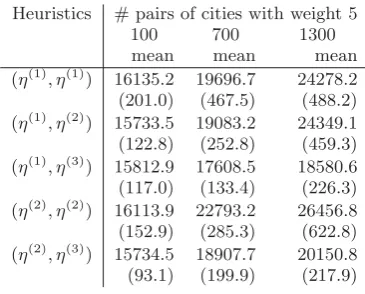
Table 1: Experiment 1: Average solution quality and standard deviation (in brackets) of PACO with diﬀerent heuristics for berlin52 instance with diﬀer-ent number of pairs of cities with weight 5

Heuristics # pairs of cities with weight 5

100 700 1300

mean mean mean

(η(1), η(1)) 16135.2 19696.7 24278.2

(201.0) (467.5) (488.2)

(η(1), η(2)) 15733.5 19083.2 24349.1

(122.8) (252.8) (459.3)

(η(1), η(3)) 15812.9 17608.5 18580.6

(117.0) (133.4) (226.3)

(η(2), η(2)) 16113.9 22793.2 26456.8

(152.9) (285.3) (622.8)

(η(2), η(3)) 15734.5 18907.7 20150.8

(93.1) (199.9) (217.9)

pair of cities has weight 0.2 or weight 5. For the third

experi-ment 2-CT-TSP instances were created where the weight for each pair of cities was chosen randomly with uniform

prob-ability from the interval [1,5].

For deﬁning the distances dij we used the TSP test

in-stances berlin52 and eil101 from the standard benchmark library TSPLIB [16]. Note, that the total number of cities (pairs of cities) is 52 (respectively 1326) for berlin52 and 101 (respectively 5050) for eil101. The test parameter val-ues that were used are (if not stated otherwise): 10 ants

per iteration, population size |P| = 5, α = 1, β = 5,

τinit = 1/(n−1), τsolution = 0.3, andτelite = 0.2. Note,

that parameter values α= 1 andβ = 5 are typically used

in ACO algorithms for the TSP (e.g., [4]) and it has been shown that a small population size works well for PACO and the TSP ([7]). Each test run was done over 1000 iterations and has been repeated 50 times. The results given in Section 6 are averages over these 50 runs.

The influence of the different heuristics was tested. In particular, it was tested how important it is to use a heuristic for the construction of the second tour that takes the first

tour into account. Therefore, heuristics η(1) and η(2) have

been tested for the construction of the ﬁrst tour of an ant

and all three heuristicsη(1),η(2), andη(3)have been tested

for the construction of the second tour. We use notation (η(i), η(j)) for a test run where heuristicη(i)is used for the

construction of the ﬁrst tourπ1and heuristicη(j)is used for

the construction of the second tourπ2,i, j∈ {1,2,3}.

6. RESULTS AND DISCUSSION

Table 1 shows the results of the PACO for the 2-CT-TSP instances of Experiment 1 when using the different heuristics and for different number of pairs of cities with weight 5. The relative quality of PACO with the different pairs of heuristics

can also be seen in Figure 1. The pair of heuristics (η(1), η(3))

is best for nearly all diﬀerent number of pairs of cities with weight 5 that have been tested. An exception is the case with a small number of only 100 pairs of cities with weight 5. In

this case the pairs of heuristics (η(1), η(1)) and (η(1), η(2))

perform best. Thus, most often it is best when the ﬁrst

(5)

0% 10% 20% 30% 40%

0 500 1000

number of pairs of cities with weight 5

relativ

e solution quality

(η(2),η(3)) (η(2)_,_η(2)₎

(η(1),η(3)) (η(1)_,_η(2)₎

(η(1)_,_η(1)₎

0% 20% 40% 60%

0 300 600 900

relativ

e solution quality

(η(2),η(3)) (η(2)_,_η(2)₎

(η(1₎_,_η₍3₎₎

(η(1),η(2)) (η(1)_,_η(1)₎

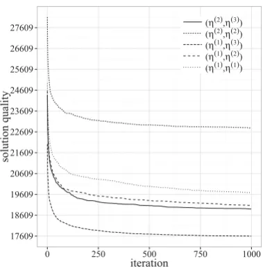
Figure 1: Experiment 1: relative average solution quality for diﬀerent number of pairs of cities with weight 5, top: berlin52, bottom: eil101

17609 18609 19609 20609 21609 22609 23609 24609 25609 26609 27609

0 250 500 750 1000

iteration

solution quality

(η(2),η(3))

(η(2)_,_η(2)₎

(η(1)_,_η(3)₎

(η(1),η(2))

(η(1)_,_η(1)₎

Figure 2: Experiment 1: convergence behaviour of PACO for berlin52 instance with 700 pairs of cities with weight 5

for the second tourπ2the heuristicη(3)which considers the

weights and considers also which pairs of cities are already

included in tour π1. Clearly, in the extreme cases when all

edges have the same weight heuristicsη(1)andη(2) become

equal. In the experiments usingη(1) instead ofη(2) for the

ﬁrst tourπ1is always better. The solution quality diﬀerence

between using the two heuristics forπ1 is particularly large

when only few pairs of cities with weight 1 exist. When using

η(1)for tourπ1 it is nearly always better to useη(3) forπ2

instead of using η(2). The results for the eil101 instances

are very similar to the corresponding results for berlin52 instances (see Figure 1).

Figure 2 gives an example that shows the convergence be-haviour of PACO for the case of 700 pairs of cities with weight 5. It can be seen that the quality diﬀerences between the diﬀerent PACO versions occur already after a few iter-ations and that the algorithms have mostly converged after 1000 iterations.

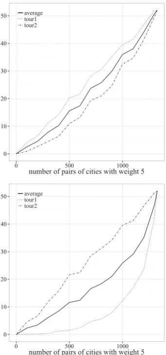
The number of pairs of cities of weight 5 that are included in the solutions of Experiment 1 are shown in Figure 3 for

PACO with heuristics (η(1), η(3)) and (η(2), η(3)). Note, that

in the extreme cases of instances with only pairs of cities with weight 1 and with only pairs of cities with weight 5 each tour includes zero, respectively 52, pairs of cities with

weight 5. Since heuristicη(1)does not consider the weights,

the number of pairs of cities with weight 5 in the ﬁrst tour

π1 increases linearly with the total number of pairs of cities

with weight 5 in the problem instance. The eﬀect of using

heuristicη(3)for the second tourπ2is that the second tour

contains less pairs of cities with weight 5. When heuristic

η(2)is used for tourπ1 there are clearly fewer pairs of cities

with weight 5 in tour π1. This holds in particular for

in-stances with a medium total number of pairs of cities with weight 5. In these cases it is relatively easy to avoid using pairs of cities with weight 5 for the second tour.

Table 2 shows the quality of the following variants of

(6)

re-0 10 20 30 40 50

0 500 1000

average tour1 tour2

0 10 20 30 40 50

0 500 1000

average tour1 tour2

Figure 3: Experiment 1: average number of pairs of cities with length 5 in the ﬁrst tour π1 and the

second tourπ2, for PACO with (η(1), η(3)) (top) and

(η(2), η(3))(bottom)

Table 2: Experiment 1: average solution quality of PACO for berlin52 instance with diﬀerent num-ber pairs of cities with weight 5, for each version of PACO also the best combination of heuristics is shown

Algorithm # pairs of cities with weight 5

version 100 700 1300

τelite= 0.2 16620 18771 19843

β= 2 (η(1), η(3)) (η(1), η(3)) (η(1), η(3)) τelite= 0.2 16054 18201 19408

β1= 5,β2= 2 (η(2), η(3)) (η(1), η(3)) (η(1), η(3)) τelite1= 0.2 15824 17658 18644

τelite2= 0 (η(1), η(2)) (η(1), η(3)) (η(1), η(3))

0% 20% 40% 60%

0 500 1000

relativ

e solution quality

(η(2₎_,_η₍3₎₎

(η(2),η(2)) (η(1)_,_η(3)₎

(η(1),η(2)) (η(1)_,_η(1)₎

Figure 4: Experiment 2 (each pair of cities has weight w = 0.2 or w= 5): relative average solution quality for diﬀerent number of pairs of cities with weight 5

duced, 2)β= 5 is used for the construction of tourπ1 and

β= 2 is used for the construction of tourπ2, i.e., the

inﬂu-ence of the heuristic is smaller for the second tour, and 3) the elitist solution is only used for the construction of the ﬁrst

tourπ1but not for the second tourπ2(i.e., a diﬀerent value

for parameterτelite was used for π1 (τelite1 = 0.2) and π2

(τelite2 = 0)). One hypothesis why PACO variants (2) and

(3) might be good is that the construction of the second tour should depend on the first tour that has already been con-structed by the ant. The reason is that some pairs of cities should be avoided for the second tour that are included al-ready in the first tour. In these cases a strong influence of a heuristic or of the elitist solution might lead the ants in the wrong direction. However, the results show that this hypothesis does not hold. None of the three PACO variants (1) - (3) results in a better solution quality.

The results of Experiment 2 where each pair of cities has

either weight 0.2 or 5 are shown in Figure 4. For small

and medium numbers of pairs of cities with weight 5 the relative solution quality of the PACO versions shows diﬀer-ences to the results of Experiment 1. For less than 800 pairs

of cities with weight 5 heuristics (η(2), η(3)) are better than

(η(1), η(3)). Heuristics (η(2), η(2)) is the worst combination

for each problem instance in Experiment 1. However, in

Experiment 2 (η(2), η(2)) is the second best combination for

small and medium numbers (200 - 600) of pairs of cities with weight 5. This shows, that the existence of a large enough

number of pairs of cities with a small weight (<1) is useful

for a heuristic that prefers pairs of cities with small weight

for tourπ2 when they are already included in the ﬁrst tour

π1.

For the evaluation of Experiment 3 all pairs of cities where

classiﬁed with respect to their weight. Four classes are

considered with weights in one of the following intervals: [1.0,2.0), [2.0,3.0), [3.0,4.0), and [4.0,5.0]. Figure 5 shows the fraction of pairs of cities in the diﬀerent classes that are

included in the ﬁrst tourπ1and in the second tourπ2. It can

(7)

tourπ1is nearly the same in all weight classes when heuristic

η(1)is used for the construction ofπ1. This is diﬀerent when

heuristicη(2)is used for the construction ofπ1. In that case,

pairs of cities with small distance are preferred and a higher

percentage of pairs of cities in class [1.0,2.0) is contained in

π1 than for pairs of cities in class [4.0,5.0] (the percentage

for the former class is approximately 15 times higher). This

holds also for tourπ2when heuristicη(2)is used and this

re-sult is relatively independent from the heuristic that is used for the ﬁrst tour.

The results are very diﬀerent whenη(3)is used for the

con-struction of the second tourπ2. If in that caseη(2)is used for

tourπ1, the percentage of pairs of cities in tourπ2 is much

higher for class [4.0,5.0] than for class [1.0,2.0). The reason

is that heuristicη(3)can diﬀerentiate if a pair of cities with

large weight is included inπ1 or not. If not, such a pair of

cities can be chosen for tourπ2 without the disadvantage of

increased costs. When heuristicη(3) is used for the second

tourπ2 together with heuristicη(1)for tourπ1 the

percent-age of pairs of cities inπ2 is smaller for class [4.0,5.0] than

for class [1.0,2.0). Here, tourπ1includes already many pairs

of cities with small distance and large weight. These pairs

of cities should not be chosen for tourπ2.

7. CONCLUSIONS

A new version of the Traveling Salesperson problem (TSP) which is called the Combined Tours TSP (CT-TSP) was defined in this paper. The aim of the CT-TSP is to find several (cyclic) tours that connect given cities such that each city is contained exactly once in each tour. The total costs of all tours should be minimum. The problem is that the costs of one tour may depend on the other tours. In this paper the particular version of CT-TSP where two tours are sought was studied (2-CT-TSP). For the studied cost function each pair of cities has a length and a weight. The quality of a solution of the corresponding 2-CT-TSP depends on the total lengths of both tours but also on the weights of the included pairs of cities. The weights are used to indicate if it is advantageous or disadvantageous when a pair of cities is contained in both tours. A Population based Ant Colony Optimization (PACO) algorithm was applied for solving the 2-CT-TSP. It was investigated how different heuristics that the ants use for the construction of the tours influence the solution quality. It was shown that it can be important that an ant uses a different heuristic for the construction of the first tour and the second tour. In particular, the heuristic for the construction of the second tour should use the knowledge about which pairs of cities are included in the first tour.

8. ACKNOWLEDGMENTS

This work has been supported by the European Social Fund (ESF) and the Free State of Saxony within the Nach-wuchsforschergruppe ”Schwarm-inspirierte Verfahren zur Op-timierung, Selbstorganisation und Ressourceneﬃzienz”.

9. REFERENCES

[1] T. Bektas: The multiple traveling salesman problem: an overview of formulations and solution procedures. OMEGA: The International Journal of Management Science 34(3): 209-219, 2006.

[2] Y.J. Costa Salas, R.A. Led´on, N.I. Coello Machado, A.

Now´e: Multi-type ant colony system for solving the

1.9 5.26

1.96 1.82 2.07

0.69 2.06

0.25

0 2 4 6

[1.0,2.0) [2.0,3.0) [3.0,4.0) [4.0,5.0]

percentage used pairs of cities

(η(1),η(2))−tour1 (η(1),η(2))−tour2

2.01 2.6

2.03 1.95 2.02 1.8 1.95

1.65

0 1 2 3

[1.0,2.0) [2.0,3.0) [3.0,4.0) [4.0,5.0]

(η(1),η(3))−tour1 (η(1),η(3))−tour2

5.08 5.07

1.79 1.78

0.81 0.81 0.36 0.36

0 2 4 6

[1.0,2.0) [2.0,3.0) [3.0,4.0) [4.0,5.0]

(η(2),η(2))−tour1 (η(2),η(2))−tour2

5.08

1.44 1.83 1.76

0.81 2.28

0.32 2.51

0 2 4 6

[1.0,2.0) [2.0,3.0) [3.0,4.0) [4.0,5.0]

(η(2),η(3))−tour1 (η(2),η(3))−tour2

Figure 5: Experiment 3 (each pair of cities has a weight in[1,5]): average percentage of pairs of cities used in the diﬀerent weight classes by the ﬁrst tour

(8)

multiple traveling salesman problem. Rev. T´ec. Ing. Univ. Zulia., 35(3): 311 - 320, 2012.

[3] Y.J. Costa Salas, W.A. Sarache Castro: An alternative solution for the repair of electrical breakdowns after natural disasters based on ant colony optimization. DYNA, 81(186): 304-310, 2014.

[4] M. Dorigo, L.M. Gambardella: Ant Colony System: A Cooperative Learning Approach to the Traveling Salesman Problem. IEEE Transactions on Evolutionary Computation, 1:53-66, 1997.

[5] M. Fischetti, J.J. Salazar-Gonzalez, P. Toth: A Branch and Cut Algorithm for the Symmetric Generalized Traveling Salesman Problem. Operations Research, 45(3):378-394, 1997.

[6] M. Fischetti, P. Toth: An Additive Approach for the Optimal Solution of the Prize-Collecting Traveling Salesman Problem. In Vehicle Routing: Methods and Studies. B.L. Golden, A.A. Assad (eds.).

North-Holland, Amsterdam, 319-343, 1988. [7] M. Guntsch, M. Middendorf: A Population Based

Approach for ACO. Proc. 2nd European Workshop on Evolutionary Computation in Combinatorial

Optimization (EvoCOP-2002), LNCS 2279, 72-81, 2002. [8] G. Gutin, A.P. Punnen (Eds): The Traveling Salesman

Problem and Its Variations. Springer, Combinatorial Optimization Series, Vol. 12, 2007.

[9] J. LaRusic: The bottleneck traveling salesman problem

and some variations.M.Sc. thesis, Department of

Mathematics, Simon Fraser University , 2010.

[10] M.A. Liang: Ant Colony Optimization for Bottleneck TSP. Computer Engineering, 9: 24-25, 2001.

[11] Y.-C. Lin, M. Clauß, M. Middendorf: Simple Probabilistic Population Based Optimization. IEEE Transactions on Evolutionary Computation, early access article, DOI 10.1109/TEVC.2015.2451701, 2015. [12] R. Matai, S.P. Singh, M.L. Mittal:Traveling Salesman Problem: An Overview of Applications, Formulations, and Solution Approaches. In: D. Davendra (ed.), Traveling Salesman Problem, Theory and Applications, 2010.

[13] S. Oliveira, M. S. Hussin, T. St¨utzle, A. Roli, M.

Dorigo: A detailed analysis of the population-based ant colony optimization algorithm for the TSP and the QAP. Proc. Genetic and Evolutionary Computation Conference (GECCO-2011), 13-14, 2011.

[14] A. Plebe, A.M. Anile: A Neural-Network-Based Approach to the Double Traveling Salesman Problem. Neural Computation, 14(2): 437-471, 2002.

[15] J.-Y. Potvin: A Review of Bio-Inspired Algorithms for Vehicle Routing. In: F.B. Pereira, J. Tavares (eds.), Bio-inspired Algorithms for the Vehicle Routing Problem, Studies in Computational Intelligence, Vol. 161, 1-34, 2009.

[16] G. Reinelt: TSPLIB. http://comopt.iﬁ.uni-heidelberg.de/software/TSPLIB95.

[17] M. Reihaneh, D. Karapetyan: An Eﬃcient Hybrid Ant Colony System for the Generalized Traveling Salesman Problem. Algorithmic Operations Research, 7: 21-28, 2012.

[18] X. Shi, L. Wang, Y. Zhou, Y. Liang: An Ant Colony Optimization Method for Prize-collecting Traveling

Salesman Problem with Time Windows. Proc. Fourth International Conference on Natural Computation (ICNC ’08), 480 - 484, 2008.

[19] T. Weise, R. Chiong, J- L¨assig, K. Tang, S. Tsutsui,

W. Chen, Z. Michalewicz, X. Yao: Benchmarking Optimization Algorithms: An Open Source Framework for the Traveling Salesman Problem. IEEE

Computational Intelligence Magazin, 9(3):40-52, 2014. [20] J. Yang, X. Shi, M. Marchese, Y. Liang: An ant colony

optimization method for generalized TSP problem. Progress in Natural Science, 18:1417-1422, 2008. [21] B. Yu , Z.Z. Yang: An ant colony optimization model:

The period vehicle routing problem with time windows. Transportation Research Part E: Logistics and

Transportation Review, 47(12):166-181, 2011. [22] W. Zhou, P. Yao: An Improved Ant Colony

A Population Based ACO Algorithm for the Combined Tours TSP Problem