SY ST E M A T IC A P P R O A C H E S TO SE T T IN G C O N SE R V A T IO N P R IO R IT IE S U SIN G S P E C IE S ’ D IST R IB U T IO N D A T A .
Melanie Kershaw
Thesis submitted for the degree of Doctor of Philosophy, University of London.
September 1996.
Institute of Zoology, Regent’s Park, London. &
ProQuest Number: 10106659
All rights reserved
INFORMATION TO ALL USERS
The quality of this reproduction is dependent upon the quality of the copy submitted.
In the unlikely event that the author did not send a complete manuscript and there are missing pages, these will be noted. Also, if material had to be removed,
a note will indicate the deletion.
uest.
ProQuest 10106659
Published by ProQuest LLC(2016). Copyright of the Dissertation is held by the Author.
All rights reserved.
This work is protected against unauthorized copying under Title 17, United States Code. Microform Edition © ProQuest LLC.
ProQuest LLC
789 East Eisenhower Parkway P.O. Box 1346
ABSTRACT.
The need to select priority areas for conservation action stems from the fact that
throughout the world, human activity is increasingly resulting in the loss or irreversible
alteration of natural ecosystems and their component species. Since there are not the
resources to protect all species and communities and because diversity is not distributed
equally, it has become necessary to select areas for conservation based on an assessment
of the worthiness of a site compared with other sites or the countryside as a whole.
The setting of such priorities for conservation is a difficult task and in the past has been
highly subjective with no clear objective or targets. Recently there have been moves
towards a more systematic approach to the selection of conservation areas, with the aim
of representing the widest possible range of the biotic diversity as efficiently as possible.
However, while this aim may be universal, its practical implementation and its
implications are unclear.
At a fundamental level there are three problems underlying attempts to make systematic
selections of priority areas for conservation: (i) What is biodiversity and what are we
trying to conserve? (ii) What surrogate measure can be used for overall diversity? and
(iii) how should priority sites be selected using this information?
These three problems are evaluated and possible solutions investigated for two extensive
data sets of distribution data. The first is for Afrotropical antelopes and includes
information on species richness, taxonomic diversity, richness of threatened species and
degree of rarity, for 249 areas in Africa. The second data set consists of distribution data
for birds, carnivores and ungulates and plants in KwaZulu Natal, South Africa.
Using these data I discuss the different possible definitions of what constitutes
biodiversity and investigate the consequences of using different components of
biodiversity for selecting priority areas for conservation. These components include
simple species richness, taxonomic diversity, threatened species, endemic species and
The second problem associated with setting priorities for conservation is that since we
do not know how many species exist or how they are distributed it is necessary to have
some sort of surrogate measure that can be used to evaluate the importance of areas for
a wide range of biotic diversity. Different potential surrogate measures, including
indicator groups, higher taxon richness, endemic species and habitat representativeness
are evaluated in terms of their ability to represent a range of diversity across a variety of
taxa.
Finally, once the diversity value of different sites has been determined it is necessary to
select a network of priority areas to represent the diversity. This requires some sort of
site selection method. Simple scoring approaches where the top ranking sites for
particular diversity criteria are compared to more sophisticated techniques using iterative
ACKNOWLEDGEMENTS.
Many people have provided data and computer software for use in this work. I am very
grateful to Paul Williams for making his WORLDMAP software available and for many
useful discussions concerning area selection algorithms. I should also like to thank my
supervisor, Georgina Mace, as well as Dick Vane-Wright, Chris Humphries, Josh
Ginsberg, Âke Berg, John Prendergast, Rachel Quinn and Blair Csuti for helpful ideas
over the past few years. John Prendergast, Paul Williams, Andrew Balmford, Tim
Coulson and Steve Albon kindly commented on earlier drafts of this thesis. Rod East
provided helpful comments concerning the Afrotropical antelopes analysis.
On the computing front I should like to thank Adrian Fisher for helping with the area
selection algorithms and for teaching me to program. Steve Wilkinson provided advice
on the use of CANOCO and how to understand ordination biplots.
The director (research) of the National Botanical Institute, Pretoria is thanked for the
use of data produced by the Pretoria National Herbarium Computerised Information
System (PRECIS). These data consisted of all quarter degree distribution records for
plant taxa collected in KwaZulu Natal, South Africa. Temperature data for KwaZulu
Natal was kindly supplied by Prof. R E. Schulze, University of Natal. Ingrid Figenschou,
Computing Centre for Water Research, University of Natal provided the precipitation
data for KwaZulu Natal. The 15 x 15 minute precipitation data were extracted from a
data set generated by Steve Lynch, Dept, of Agricultural Engineering, University of
Natal. The steering committee responsible for this project consisted of the following
persons: Mr D.W.H. Consens (Water Research Commission chairman), Mr P.W.
Weidman (WRC secretary), Dr P.J.T. Roberts (WRC), Prof. P. Meiring (University of
Natal), Mr F.J.Kruger (Dept of Environment Affairs), Mr J.F. Erasmus (Dept of
Agriculture & Water Supply), Dr P.T. Adamson (Dept, of Water Affairs), Mr F. Viljoen
(Dept, of Environment Affairs). The financing of the project by the WRC and the
contributions of members of the steering committee is acknowledged gratefully. This
project of five years duration was only possible with the cooperation of many individuals
of Environment Affairs, South African Weather Bureau, Dept, of Agriculture and Water
Supply, Soil and Irrigation Research Institute, University of Natal, Pietermaritzburg,
Computer Services Division, University of Witwatersrand erstwhile Hydrological
Research Unit, Prof. D C. Midgley, Dr W.V. Pitman, Dept, of Environment Affairs, S.A.
Forestry Research Institute, J. Bosch, F. Rogers, South African Sugar Association
Experiment Station, G. Thompson, M. Murdoch, R. Harding, Natal Parks Board,
Organised Agriculture, Public of South Africa, Dept of Geography, University of Natal,
Pietermaritzburg, A.W. Seed, H.M.M. Wills, The Computing Centre for Water Research,
the Water Research Commission, Dr R. Sparks, Prof. W. Zucchnini, Prof. G. Pegram,
A. Lonergan, S. Piper, Dept, of Land Surveying and Mapping, University of Natal,
Durban, G. Angus, S. Dunsmore, J. Garland, B. Gaydon, W. George, M. Maharaj, E.
Murgatroyd, S. Neuwirth, C O. Mahoney, H. Tarboton, K. Temple, J. Whyte, K. Wiercx,
N. Wijnberg, J. Swanepoel, K. Fismer, M. Gorven and A. Kure.
I should particularly like to thank Adrian for aU his support over the past three years (and
persuading me not to give up on the thesis), my parents for their encouragement (and for
daring to proof read some of the chapters), Marcus for being very tolerant of all the mess
in the flat and everyone at WWT for distracting me for the last year so I didn’t get a
Declaration.
I declare that the work contained in this thesis is my own. Some of the work contained
in Chapter 2 has been published jointly with Paul Williams and Georgina Mace (Kershaw,
M., Williams, P.H & Mace, G.M. 1994. Conservation of Afrotropical antelopes:
consequences and efficiency of using different site selection methods and diversity
criteria. Biodiversity and Conservation 3, 354-372.). This paper was written by me and
the analysis in the paper was also carried out by myself. Results presented in Chapter 5
are also published (Kershaw, M., Mace, G.M. & Williams, P.H. 1995. Threatened status,
rarity and diversity as alternative selection measures for protected areas: a test using
Afrotropical antelopes. Conservation Biology 9, 324-334.). Again the analysis was done
by myself and I wrote the paper. Some of the data from KwaZulu Natal have been
published with Georgina Mace (Mace, G.M. & Kershaw, M. In press. Extinction Risk
and Rarity on an Ecological Timescale. In The Biology o f Rarity, (eds. W.E. Kunin &
K.J. Gaston), pp 130-149, 1997.). The results of the analyses contained in this
publication are not included in this thesis. Some of the work in Chapter 6 is also
published jointly (Csuti, B., Polasky, S., Williams, P H., Pressey, R.L, Camm, J.D.,
Kershaw, M., Kiester, A.R. Downs, B., Hamilton, R., Huso, M & Sahr, K. In press.
Biological Conservation. A comparison of reserve selection algorithms using data on
terrestrial vertebrates in Oregon.). Chapter 6 only includes the analysis which I did for
Contents.
Title page... 1
Abstract... 2
Acknowledgements... 4
Declaration... 6
Contents...7
List of tables...9
List of figures... 12
Chapter 1. General Introduction... 16
Chapter 2. A comparison of the efficiency of alternative area selection criteria at representing different biodiversity attributes... 44
Introduction... 44
Methods... 46
Results... 58
Discussion... 75
Conclusions...87
Chapter 3. Quantifying patterns of richness and spatial turnover: what makes a good surrogate measure for wholesale biodiversity?...88
Introduction... 88
Methods... 94
Results...112
Discussion... 143
Conclusions... 156
Introduction...157
Methods... 161
Results... 165
Discussion... 177
Conclusions... 184
Chapter 5. A comparison of the efficiency of different iterative reserve selection algorithms... 185
Introduction...185
Methods... 187
Results... 192
Discussion... 203
Conclusions...210
Chapter 6. General Discussion... 211
List of Tables.
Table 2.1. Numbers of species, threatened species, endemic species and restricted-range species in each of the different taxonomic groups in the data set for KwaZulu Natal.
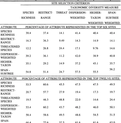
Table 2.2. Percentage of different diversity attributes represented in the top six and twelve sites selected using alternative diversity criteria for Afrotropical antelopes.
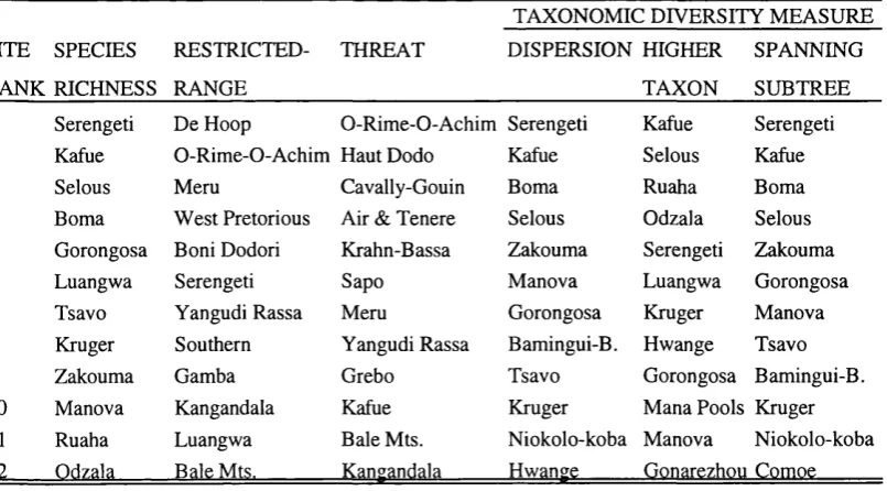
Table 2.3. Top ranking sites according to the alternative diversity criteria for Afrotropical antelopes.
Table 3.1. List of the environmental variables included in the CCA analysis for birds, mammals and grasses in KwaZulu Natal.
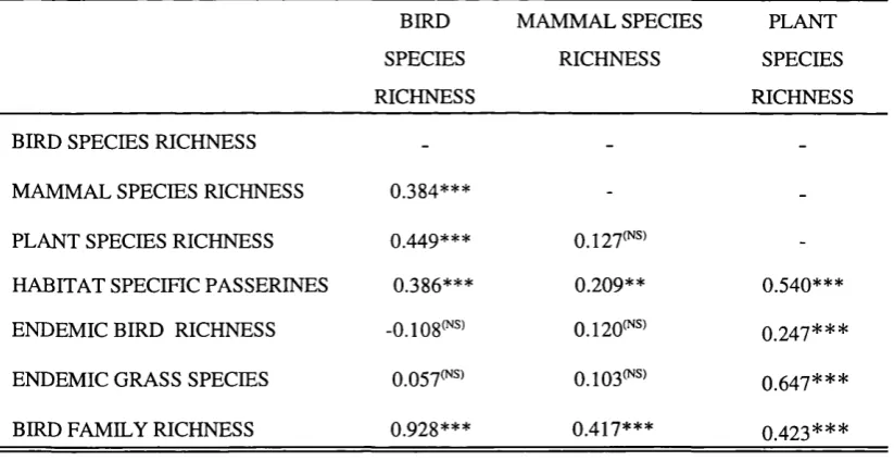
Table 3.2. Correlation coefficients (r) between species richness of quarter degree grid cells (n=166) for different groups in KwaZulu Natal.
Table 3.3. Percentage overlap of top sites for bird, mammal and plant species richness with sites selected using alternative diversity criteria.
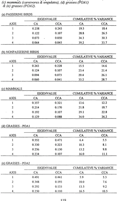
Table 3.4. Eigenvalues & cumulative percentage variance explained by the first four axes extracted by correspondence analysis compared to canonical correspondence analysis of sites in KwaZulu Natal, southern Africa based on (a) passerine birds, (b) nonpasserine birds, (c) mammals (carnivores & ungulates), (d) grasses (Poal) and (e) grasses (Poa2).
Table 3.5. Eigenvalues for the first four axes extracted by canonical correspondence analysis for each group (passerines, nonpasserines, mammals and grasses (Poal & Poa2)), with their significance levels calculated from 99 Monte Carlo permutations.
Table 3.6a. Interset correlations of the first CCA axis with environmental variables, arranged in rank order for each taxon.
Table 3.6b. Interset correlations of the second CCA axis with environmental variables, arranged in rank order for each taxon.
Table 3.7. Species turnover values for birds, mammals & plants along fourteen east-west transects in KwaZulu Natal, measured using two alternative methods (Harrison e. al. 1992 & Whittaker 1960 - see text for explanation).
calculated for habitat specific and habitat generalist passerine species separately using the Harrison et al. (1992) measure of species turnover.
Table 3.10. Mean pairwise similarity (CCJ (xlOO) for birds and plants, between 168 pairs of sites from the same dominant habitat type, and 168 pairs of sites from different dominant habitat types.
Table 3.11. Percentage of species represented in the top eight sites (hotspots) selected using alternative diversity criteria.
Table 4.1. Number of sites needed to represent all species using two alternative sites selection methods (selection of top sites (scoring) and an iterative richness algorithm) & efficiency of iterative site selection methods compared to the selection of top scoring sites for birds, mammals and plants in KwaZulu Natal and Afrotropical antelopes.
Table 4.2. Numbers (%) of species represented in the first eight sites (for KwaZulu Natal taxa) or first twelve sites (Afrotropical antelopes) selected by the two alternative selection methods.
Table 4.3. First twelve sites selected to represent Afrotropical antelopes using two alternative selection methods (scoring versus an iterative richness algorithm). The cumulative number of species that would be represented as sites are added to the network is also given.
Table 4.4. First eight sites selected to represent bird species in KwaZulu Natal using two alternative selection methods (scoring versus an iterative richness algorithm). The cumulative number of species that would be represented as sites are added to the network is also given. Sites are coded as letters corresponding to the west-east and north-south position of the quarter degree grid cell.
Table 4.5. First eight sites selected to represent mammal species in KwaZulu Natal using two alternative selection methods (top sites versus an iterative richness algorithm). The cumulative number of species that would be represented as sites are added to the network is also given.
Table 4.6. First eight sites selected to represent plant species in KwaZulu Natal using two alternative selection methods (top sites versus an iterative richness algorithm). The cumulative number of species that would be represented as sites are added to the network is also given.
Table 4.7. Effect of having some sites already preassigned to the site network on the efficiency of an iterative selection of sites for Afrotropical antelopes.
preassigned sites (2, 5, 10 & 15). P values give the two-tailed significance level.
Table 4.9. t-tests for the difference between the mean number of sites needed to represent all Afrotropical antelope species with no sites preassigned to the network compared to when different numbers of sites, of varying richness are preassigned. P values give the two-tailed significance level.
Table 4.10. Comparison of the ability (in terms of number and percentage of species) of different site selection methods at representing threatened and endemic species for birds, mammals and plants in KwaZulu Natal.
Table 4.11. Comparison of the ability (in terms of % of species/diversity represented) of different site selection methods at representing threatened species, restricted- range species and taxonomic diversity for Afrotropical antelopes.
Table 5.1. Number of sites needed to represent all species using four different iterative algorithms. Numbers in brackets denote the number of sites that were ‘redundant’ following the backtracking procedure which was applied to the richness algorithms for the KwaZulu Natal taxa.
Table 5.2. Efficiency of the different iterative algorithms.
Table 5.3. Sites selected by the different iterative algorithms for Afrotropical antelopes.
Table 5.4. Number of species that are represented by each of the alternative iterative algorithms when the number of sites that can be selected is limited.
Table 5.5. Number of sites needed to include all species in the Oregon data set using four different iterative algorithms (richness, rarity I, rarity II & rarity III) compared to the optimal solution as derived from integer programming.
List of Figures.
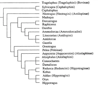
Figure 2.1. Classification of Afrotropical antelopes (based on Gentry 1992) used to derive taxonomic diversity measures in WORLDMAP.
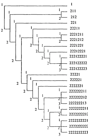
Figure 2.2. Example illustrating the formulation of codes used to enter a taxonomic hierarchy into WORLDMAP. The program weights different faunas according to the number of taxa and number of internodes subtended by the included species.
Figure 2.3. Map of southern Africa showing the location of KwaZulu Natal.
Figure 2.4. Ability of alternative site selection criteria (x axis) at representing different biodiversity attributes of Afrotropical antelopes: (a) species richness; (b) restricted-range richness; (c) threatened species richness; (d) dispersion-weighted taxonomic diversity, (e) higher-taxon weighted diversity & (f) spanning-subtree weighted taxonomic diversity.
Figure 2.5. Ability of alternative site selection criteria (x axis) at representing different biodiversity attributes of birds in KwaZulu Natal: (a) species richness; (b) threatened species richness; (c) endemic species richness & (d) restricted-range richness.
Figure 2.6. Ability of alternative site selection criteria (x axis) at representing different biodiversity attributes of mammals in KwaZulu Natal: (a) species richness; (b) threatened species richness & (c) restricted-range species richness.
Figure 2.7. Abihty of alternative site selection criteria (x axis) at representing different biodiversity attributes of plants in KwaZulu Natal: (a) species richness; (b) threatened species richness & (c) restricted-range species richness.
Figure 2.8. Ability of alternative site selection criteria (x axis) at representing different biodiversity attributes of grasses in KwaZulu Natal: (a) species richness; (b) endemic species richness & (c) restricted-range species richness.
Figure 2.9. Location of the top eight sites selected by the alternative diversity criteria for birds in KwaZulu Natal.
Figure 2.10. Location of the top eight sites selected by the alternative diversity criteria for mammals in KwaZulu Natal.
Figure 2.11. Location of the top eight sites selected by the alternative diversity criteria for plants (all species) in KwaZulu Natal.
Figure 2.12. Location of the top eight sites selected by the alternative diversity criteria for grasses in KwaZulu Natal.
species, but different taxonomic diversity scores as calculated by the three WORLDMAP measures.
Figure 2.13b. Cladograms showing where species from three of the antelope sites lie on the overall classification (Meshra, Harrar & Scio). Each site has three species, but different taxonomic diversity scores as calculated by the three WORLDMAP measures.
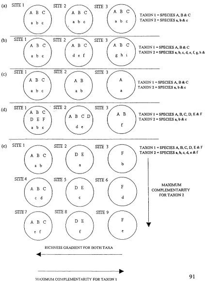
Figure 3.1. Five hypothetical groups of sites (a-e) showing different levels of species richness and spatial turnover (complementarity) for two taxa.
Figure 3.2. Map of KwaZulu Natal showing the different habitat types, redrawn from Rowe-Rowe 1992a.
Figure 3.3. Concordance of top sites for bird, mammal & plant species richness in quarter degree squares in KwaZulu Natal, southern Afi*ica. The top eight squares for each taxon are shown.
Figure 3.4. Relationship between bird species richness and bird family richness of quarter degree squares in KwaZulu Natal, southern Africa.
Figure 3.5. Ordination diagram based on canonical correspondence analysis of passerine distribution data in 166 quarter degree squares in KwaZulu Natal, with respect to the environmental variables..
Figure 3.6. Ordination diagram based on canonical correspondence analysis of mammal distribution data in 166 quarter degree squares in KwaZulu Natal, with respect to the environmental variables.
Figure 3.7. Ordination diagram based on canonical correspondence analysis of grass (POAl) distribution data in 166 quarter degree squares in KwaZulu Natal, with respect to the environmental variables.
Figure 3.8. Ordination diagram based on canonical correspondence analysis of passerine distribution data in KwaZulu Natal with respect to the environmental variables. Each of the 195 breeding passerine landbird species is shown as the centroid (A) representing the species’ optima in 2-dimensional space in the ordination.
Figure 3.9. Ordination diagram based on canonical correspondence analysis of passerine distribution data in KwaZulu Natal with respect to the environmental variables. Each of the endemic, breeding, passerine landbird species is shown as the centroid (A) representing the species’ optima in 2-dimensional space in the ordination.
species is shown as the centroid (A) representing the species’ optima in 2- dimensional space in the ordination.
Figure 3.11. Ordination diagram based on canonical correspondence analysis of passerine distribution data in KwaZulu Natal with respect to the environmental variables. Each of the threatened, breeding, passerine landbird species is shown as the centroid representing the species’ optima in 2-dimensional space in the ordination.
Figure 3.12. Ordination diagram based on canonical correspondence analysis of nonpasserine distribution data in KwaZulu Natal with respect to the environmental variables. Each of the threatened, breeding, nonpasserine landbird species is shown as the centroid representing the species’ optima in 2-dimensional space in the ordination.
Figure 3.13. Ordination diagram based on canonical correspondence analysis of passerine distribution data in KwaZulu Natal with respect to the environmental variables. Each of the habitat specific, breeding, passerine landbird species is shown as the centroid (A) representing the species’ optima in 2-dimensional space in the ordination.
Figure 3.14. Ordination diagram based on canonical correspondence analysis of grass distribution data (POA2) in KwaZulu Natal with respect to the environmental variables (omitted for clarity - see figure 3.7). Each of the endemic species is shown as the centroid (A) representing the species’ optima in 2-dimensional space in the ordination.
Figure 3.15. Ordination diagram based on canonical correspondence analysis of mammal distribution data in KwaZulu Natal with respect to the environmental variables. Each of the threatened mammal species is shown as the centroid (A) representing the species’ optima in 2-dimensional space in the ordination.
Figure 3.16. Species accumulation curves as sites are added to a site network starting with the most species rich sites and selecting subsequent sites in decreasing rank order (up to a total of 30 sites). The vertical line indicated the number of species that would be represented in the top eight sites.
Figure 3.17. Percentage of threatened species represented in the top eight sites for species richness in KwaZulu Natal for each of the taxa, plants, birds & mammals.
Figure 4.1. Locations of the first eight sites selected for birds in KwaZulu Natal by the two alternative selection methods (top-ranking sites for species richness & an iterative richness selection).
Figure 4.3. Locations of the first eight sites selected for plants in KwaZulu Natal by the two alternative selection methods (top-ranking sites for species richness & an iterative richness selection).
Figure 5.1. Locations of the first eight sites selected by the different iterative algorithms (Richness, Rarity I, Rarity II & Rarity III) for birds in KwaZulu Natal.
Figure 5.2. Locations of the first eight sites selected by the different iterative algorithms (Richness, Rarity I, Rarity II & Rarity III) for mammals in KwaZulu Natal.
Figure 5.3. Locations of the first eight sites selected by the different iterative algorithms (Richness, Rarity I, Rarity II & Rarity III) for plants in KwaZulu Natal.
CHAPTER ONE.
GENERAL INTRODUCTION. The problem.
The need to select priority areas for conservation action stems from the fact that
throughout the world, human activity is increasingly resulting in the loss or irreversible
alteration of natural ecosystems and their component species (Ehrlich 1988, Myers 1988,
Wilson 1988, Vane-Wright et al. 1991, Groombridge 1992, Grehan 1993). Since there
are not the resources to protect all species and communities and because diversity is not
distributed equally, it has become necessary to prioritise areas for conservation based on
an assessment of the worthiness of a site compared to other sites or the countryside as
a whole.
In the past area selection has been highly subjective, often on the basis of individual
species or groups of species with a high public profile, or for scenic or recreational
reasons, with no clear objective or targets for species, habitat or ecosystem conservation
(Terborgh & Winter 1983, Purdie 1987, Vane-Wright 1993). Recently there have been
moves towards a more systematic approach to the selection of conservation areas, with
the aim of representing the widest possible range of biotic diversity as efficiently as
possible (Austin & Margules 1986, Margules et al. 1988, Pressey & Nicholls 1989b, May
1990, Pressey et al. 1993, Vane-Wright et al. 1994, Williams et al. 1996b). However,
while this aim may be universal, its practical implementation and its implications in terms
of the areas that are important are unclear. Even in cases where more systematic
approaches have been used, the areas selected will depend on the attributes used to
evaluate sites, the selection method, the motive for protection, and at what level of
organisation efforts are concentrated, and aims are often distorted by economics and the
availability of land (Green 1985, Pressey 1994).
A major problem in the selection of priority areas is determining what it is that we are
trying to conserve; or more generally what is biodiversity? This will be dependent on the
1996b). Priority areas could be based on a variety of different biodiversity attributes.
For example, species richness, endemic species, taxonomic richness, genetic diversity,
threatened species, ecological type diversity and community diversity are all attributes
of biodiversity which could be used to select areas for conservation, depending on the
overall conservation goal. Additionally, since we do not fully understand how certain
attributes of biodiversity contribute to potential goals like the maintenance of
evolutionary potential or ecosystem processes and function, we cannot easily determine
how to achieve these goals. A further problem is that there is not the time nor the
resources to evaluate all aspects of biodiversity. Society has to decide what the goals for
conservation are, but this needs to be based on information about the distribution of
biodiversity attributes. The aim of the work presented in this thesis is to provide the sort
of information that can guide strategic decisions concerning the best methods to achieve
alternative biodiversity goals. If we choose to base area selection on a single goal (for
example, maximising the number of species that are represented) then we need to know
which attributes of biodiversity will and will not be incorporated. This will be particularly
important in cases where a different approach or the use of different attributes would
result in very different areas being designated as high priority (Kershaw et al. 1995).
Alternatively, it may be possible to use a technique that incorporates many different
attributes and goals explicitly.
Aims of priority areas for conservation.
Conserving a representative selection of the fuU range of biotic diversity (from genes and
species to ecosystems) is a widely cited goal (Margules & Usher 1981, Bolton & Specht
1983, Van der Ploeg 1986, Pressey & Nicholls 1989b, Bedward et al. 1992, Nilsson &
Gotmark 1992, Saetersdal et al. 1993). Representativeness was defined by Austin &
Margules (1986) as a criterion for assessing how adequately a reserve or system of
reserves represents the range of biological variation in a region. Representativeness was
seen as a priority for conservation in Britain when the government published its white
papers "Conservation of nature in England and Wales" and "National Parks and the
conservation of nature in Scotland" in 1947 following the recommendation by the Huxley
field of variation in ecosystem types (Ratcliffe 1977, Usher 1986). This lead to the key
area concept - nature reserves in Britain should centre around the safeguarding of a fairly
large number of key areas which were representative of all major types of natural and
semi-natural vegetation, their fauna and habitat conditions. The key area approach was
subsequently considered largely inappropriate and in 1966, in the Nature Conservancy
Review, which was launched to reappraise candidate sites for expansion of the National
Nature Reserve network, factors like ecosystem fragility, vulnerability to future loss due
to fragility and predicted future human pressures and irreplaceability of the ecosystem
were seen as priorities.
At an international level Dasmann (1972) recognised the need to establish a worldwide
network of reserves on a biogeographical basis. With this in mind the World
Conservation Strategy (lUCN 1980) was developed with three fundamental aims:
maintenance of essential ecological processes, preservation of genetic diversity and
sustainable utilisation of species and ecosystems (lUCN 1980). In 1992 over 150
countries signed The Convention on Biological Diversity at the United Nations
Conference on Environment and Development. Part of this convention requires
contracting parties to develop national strategies for the conservation of biodiversity. In
response to this the UK Action Plan was published, the overall goal being to ‘conserve
and enhance biological diversity within the UK and to contribute to the conservation of
global biodiversity through all appropriate mechanisms’ (DoE 1994). The Action Plan
recognises the multifaceted nature of biodiversity and objectives such as representing the
range of species, wildlife habitats and ecosystems and conserving threatened species,
ecosystems and elements characteristic of local areas are cited. As well as representing
UK biodiversity the need to conserve elements of international and global importance is
also an objective (DoE 1994).
While a widely agreed goal of priority areas might be to conserve a representative range
of the existing biotic diversity, it is not obvious how this translates practically. At a
fundamental level there are three major problems underlying attempts to make systematic
results presented in this thesis:
1. What to conserve (and can different attributes of biodiversity be conserved in the
same sites)?
2. What surrogate measures can be used to reflect overall biodiversity patterns?
3. How should biodiversity value information be used to select priority areas?
Definitions.
In order to fully review the different goals and methods for the selection of priority
conservation areas it is necessary to briefly outline some of the terminology used:
Biodiversity describes the variety and variability among living organisms and the
ecological complexes in which they occur (McNeely et al. 1990). Although biodiversity
can be considered at a number of different levels (genes, species and ecosystems), species
are the most commonly used units for evaluation and areas are usually the most practical
way of conserving biodiversity.
Attributes are those properties of a site or area which can be used to reflect its
conservation interest. They represent the currency of conservation value. For example
a site attribute might be the species that are present, or the habitat types in the site.
Criteria provide a means of expressing the attributes in such a way that they can be used
to evaluate the conservation interest of a site. For instance the list of species in a site
could be used to calculate a diversity or richness index criterion, or a rarity value
criterion.
The total area from which priority sites could be drawn is termed the region. Regional
diversity is then all the elements of biodiversity that are found in the total area.
Within a region the individual sites that are selected as priority areas together form a site
Species richness is used simply to describe the number of species present in a site or
region.
Threatened species are those species that have been included on some sort of ‘red list’,
for example, Red Data Book (lUCN 1994), indicating that they are considered
susceptible to extinction in the near future. Different degrees of threat are usually
recognised, and species may be included on red lists for a number of different reasons.
New methods for assessing global threatened species lists have been adopted (lUCN
1994) although these new criteria have yet to be applied to the majority of taxa (although
see Collar et al. 1994).
Rarity has a number of definitions and the term is used in many different ways (Magurran
1988, Gaston 1994). Rabinowitz (1981) and Rabinowitz et al. (1986) identified seven
ways to be rare based on three rarity ‘traits’ - restricted-range size, habitat specificity and
small population size.
Endemic species are those that are confined to a particular geographic region. If this
region is small then the endemic species could be classified as restricted-range and
therefore represent a form of rarity.
Complementarity is the degree to which individual areas or discrete sites contain
elements of biodiversity that are represented by other sites. Two sites containing
completely different biodiversity elements have high complementarity whilst sites
containing the same or similar elements have low complementarity.
A surrogate measure is defined as an attribute which accurately reflects the patterns of
distribution across a wide range of additional taxa or other biodiversity attributes. For
example plant species richness patterns might mirror richness patterns in a range of other
taxa so selecting areas rich in plants would also select areas of high richness for other
taxa. Plants could therefore be used as a surrogate for riehness in other taxa without
Higher taxon is used to refer to any taxonomic rank that is higher than the species level,
for example family or order.
When areas have been evaluated for biodiversity value a selection method can be applied.
The sites that are selected are priority areas. These will vary according to the attributes,
criteria and selection method used.
When sites are selected for inclusion in a network by means of taking the sites ranked
most highly on the basis of some criterion (for example, species richness score) this is
described as a scoring or ranking selection method.
A selection method that proceeds in a stepwise fashion, at each step taking account of
the attributes represented by previous site selections is termed an iterative selection
method or iterative heuristic.
The ability of a set of reserves to represent the biotic diversity of an area can be termed
the efficiency of the network (Pressey & Nicholls 1989a). This can be measured in terms
of the proportion of a total region that is required to represent all the desired attributes.
Efficiency must undoubtedly be a primary objective given the pressure on land and the
cost involved.
What to conserve (and can different attributes of biodiversity be conserved in the same sites)?
It is generally agreed that the role of protected areas is to maintain a representative
selection of the existing biotic diversity, but biodiversity does not have a simple
definition. Part of the problem may be that the word biodiversity is treated as if it were
a ‘thing’ whereas in reality it is an abstract idea. Biodiversity describes the range and
variability of all living organisms (McNeely et al. 1990). If only a subset of this
variability can be conserved or protected there is no clearly objective way of determining
which group of organisms represents the ‘most’ biodiversity. Species richness,
potential and threatened or vulnerable species are all components of biodiversity which
could be used to assess the conservation value an area. Problems will arise when a set
of areas selected to maximise one aspect of biodiversity, for example, species richness
are not the best sites for other aspects of diversity, like rare or threatened species
(Prendergast et al. 1993, Kershaw et al. 1995, Williams et al. 1996a).
Threatened species.
The ultimate goal of conservation is to prevent the extinction of species (Diamond 1976,
ICBP 1992), thus species that are threatened could be an appropriate focus for the
selection of conservation areas. Species vary in their vulnerability to extinction, so if the
aim of a reserve network is to maintain a representative selection of species diversity then
it is necessary to take account of the fact that some species are less likely to persist in the
future than others. Optimisation of the amount of biodiversity represented in reserves
could jeopardise the long term representation of biodiversity if limited resources are used
to represent common species leaving vulnerable species unprotected (Witting &
Loeschcke 1995).
Species which are not threatened or potentially threatened do not need protection
(Ratcliffe 1986). Giving these species equal weighting with species that are threatened
in the short term could affect the areas that are valued as conservation priorities
(Saetersdal 1994). However if a large number of species are ultimately threatened with
extinction then concentrating on species currently threatened or vulnerable may lead to
biases in the representation of biotic diversity in the future, especially if threatened
species tend to occur in certain taxonomic, ecological or life history groups. For example
if threatened species are more likely to be classically rare species (restricted-range, small
population size and habitat specific) then concentration on single threatened species may
lead to habitats being preserved on the basis of rare species and for these species to
therefore be over-represented in protected areas.
Also it is not possible to identify every species which is threatened or potentially
Firstly not all species are known, secondly it would be far too time consuming and
practically unrealistic to evaluate the status of all species, and thirdly, there are not the
resources to set aside areas to conserve all the species that are or are likely to become
threatened (Noss 1991). Additionally, we cannot accurately predict which species will
be subject to threatening processes in the future.
In the past some conservation efforts have revolved around last ditch attempts to save
threatened species - the so-called ‘Noah Principle’ (Heywood 1988) - for example the
Black footed ferret (Groves & Clark 1986), Red-cockaded woodpecker (Reed et al.
1988), Grizzly bear (Schaffer 1983) and Spotted owl (Barrowclough & Coats 1985).
Such an approach could result in valuable resources being channelled into ‘hopeless
cases’ rather than attempting to ensure the maintenance of species and ecosystems that
have a real chance of persistence.
Nonetheless, richness of threatened species should highlight those areas in imminent
danger of losing species and therefore most in need of protection (Rebelo & Tansley
1993). Areas could be selected that maximise the number of threatened or potentially
threatened species that would be represented. Rapoport et al. (1986) proposed a method
for the designation of optimum reserve areas based on the conservation value of each
component species, weighted towards threatened species, which in turn gave a
conservation value per unit area. Species’ values depended on the local area occupied,
geographical range, density or abundance and tendency to become extinct.
However, approaches based around maximising the number of threatened species in
protected areas have also been criticised. An analysis of the plant species listed as
threatened in New South Wales, Australia revealed that 55% were confined to one of
two distinctive ecological types (McIntyre 1992). Herb species were significantly under
represented in the threatened species list compared to their contribution to the overall
flora suggesting that being less conspicuous than trees and shrubs has lead to their under
documentation (McIntyre 1992). Eighty-four percent of the species listed as threatened
specific. Only 11% of the species were widely distributed habitat generalists. This may
indicate that widespread, but uncommon species have been overlooked in assessments
of conservation status (McIntyre 1992). These species may however be the most
demanding to conserve as they will need large areas to be set aside. In contrast endemic
species may be successfully conserved in relatively small areas (McIntyre 1992).
So while there is no doubt that threatened species are a priority for conservation,
concentrating purely on threatened species could lead to biases in the future
representation of biodiversity.
Rare species.
An alternative to focusing on species categorised as threatened is to prioritise areas on
the basis of rare species, since there is a general assumption that the rare species of today
are the extinct species of tomorrow (McIntyre 1992, Gaston 1994, Mace & Kershaw in
press). But this is not necessarily the case, especially since species can be rare for a
number of different reasons and in a number of different ways, which in turn are highly
dependent on the scale used (Rabinowitz 1981, Magurran 1988, McIntyre 1992, Gaston
1994, Saetersdal 1994). Mayr (1963) recognised that species could be rare for different
reasons - either because they are highly specialised or because they are very localised.
Rabinowitz (1981; Rabinowitz et al. 1986) classified seven different ways in which rarity
could manifest itself - a species can be rare if it is geographically restricted, if it only ever
exists in small populations or if it is habitat specific. These then give rise to seven
different combinations in which a species could be rare according to one or more of the
categories, the extreme case being a species that is geographically restricted, habitat
specific and only occurs in small populations. Such species are those which would be
considered to be classic endemics, but a species can also be rare if it is widely distributed,
a habitat generalist but only ever exists in small populations and these are the sort of
species that tend to be overlooked. It is these species that are most likely to be
unprotected if areas are selected for conservation based on classically rare, restricted-
A number of studies have looked at the distributions of various forms of rarity in different
taxonomic groups and at different scales and how this relates to the future persistence
of populations (Thomas & Mallorie 1985, Pagel et al. 1991, Kattan 1992, Saetersdal
1994). Cowling & Bond (1991) found that the species most likely to be missing from
small islands fragmented from the mainland were endemics and specialists. Similarly
Newmark (1991) found that forest-dependent understorey species in Tanzania varied
greatly in their vulnerability to fragmentation, but the most susceptible groups were rare
and forest interior species (i.e. habitat specialists). Bolger et al. (1991) found a strong
positive correlation between the relative persistence ability of a species and its density in
habitat fragments and concluded that density is a primary factor in determining a species'
relative vulnerability to extinction. Small population size was found to be the most
common reason (more important than range-size) for threatened species listing in a
recent conservation review of birds using the new lUCN threatened species criteria
(Collar et al. 1994, lUCN 1994, Mace & Kershaw in press). Given & Norton (1993)
found that the most useful criteria for prioritising threatened plant conservation in New
Zealand were population decline rate, size of largest population and habitat specificity.
Geographic distribution was a redundant criterion in that it did not account for any of the
differences between species in terms of their threat status (Given & Norton 1993).
However, population size or abundance may not always be a good measure of a species’
vulnerability. There are a number of examples where persistence has been related to
distribution - that is species with small ranges are more susceptible to extinction
(Terborgh & Winter 1983, Thomas 1991, Thomas & Mallorie 1985, ICBP 1992). A
recent study by Birdlife International found that three quarters of threatened bird species
had restricted-ranges, defined as a total range of less than 50,000km^ (ICBP 1992).
Thomas & Mallorie (1985) found that while vulnerability of Moroccan butterfly species
was related to distribution, it was not necessarily related to abundance. Similarly,
Thomas (1991) compared the geographic range of Costa Rican butterflies with their
potential ability to use human-modified habitats and found that restricted-range species
Burke & Humphrey (1987) looked at rarity as a criterion for endangerment in Florida's
fauna. Generally, initial rarity (defined as limited distribution, low local density and large
body size) was a good indicator of a species’ subsequent vulnerability (as indicated by
a species’ inclusion on threatened species lists), however there were some significant
discrepancies. Some rare species were more extinction prone than expected and likewise
some species which were not rare were threatened for other biological or economic
reasons, for example by excessive settlement within their range. For instance the bat
species Myotis grisecens was very abundant where it occurred but needed caves to breed
which were uncommon and very sensitive to disturbance. So rarity may be useful as an
initial filter for assigning conservation priorities, but it will also be necessary to consider
other factors that could affect species’ persistence.
Species that have been rare for long periods may have adaptations that allow them to
persist in a rare state (Kunin & Gaston 1993, Gaston 1994, Mace & Kershaw in press).
For example, Simberloff & Gotelli (1984) looked at the effects of insularisation on plant
species richness in the prairie-forest ecotone and found that rare species were found more
often in small sites than a random colonisation model would predict i.e., they were less
susceptible to local extinction than expected. Rare species may therefore be in less need
of protection than more common species which may lack adaptations to cope with
population reduction or fragmentation.
The scale at which rarity is defined is likely to influence those species listed and is an
important consideration when setting priorities for conservation. Species that are rare
at a local scale may be common at a regional level and vice versa. When Saetersdal
(1994) classified vascular plants in Norway according to Rabinowitz’s (1986) seven
forms of rarity, a number of the species changed rarity category depending on whether
the scale used was local (deciduous woodlands in Hordaland, western Norway) or
regional (the whole of western Norway). Sixty-seven of the 225 deciduous woodland
species that were common at the local scale fell into one of the rarity categories at the
regional level (Saetersdal 1994). Seven species were rare at the local level but common
(Saetersdal 1994).
The same effect can be seen with threatened species listings. In North America, most
states and provinces have lists of state/provincially endangered species and in Europe
individual countries have their own threatened species lists (Hunter & Hutchinson 1994).
A number of the species on these lists are there because they are peripheral species, on
the edge of their range in the country in question (Hunter & Hutchinson 1994). For
example, the South African Red Data Book for birds lists a number of species that are
on the edge of their range in southern Africa but are widespread throughout the rest of
the Afrotropics and do not feature on the global list of threatened species like the Wattle
eyed Flycatcher {Platysteira peltatd) and African Broadbill (Smithornis capensis)
(Brooke 1984, Hurford et al. 1996). Similarly, there are some species that are listed as
globally threatened yet do not appear on the South African red list because they are
common within the region, for example, the Buffstreaked Chat {Oenanthe bifasciata).
Globally rare or threatened species are likely to be the greatest priority for conservation
but there are arguments for protecting locally rare species as well. To maintain the full
range of genetic diversity may require the conservation of populations across the whole
of a species’ range and populations which are at the edge of their species’ range may also
be more able to adapt to environmental change compared to core populations (Hunter
& Hutchinson 1994). There is also the possibility that loss of populations at a local level
might affect ecosystem functioning and lead to the loss of other (possibly globally rare)
species (Hunter & Hutchinson 1994). Most conservation organisations operate within
a political framework and a system globally implemented with respect to biogeographical
regions, while ideally being more appropriate would in reality be impractical (Hunter &
Hutchison 1994).
Species richness.
A commonly used measure of biodiversity value has been simple species richness (for
example, Myers 1988, Prendergast et al. 1993, Williams et al. 1996a), but it is debatable
whether it is an adequate measure of conservation value or priority. It is attractive
species rich communities are often ecotones and not typical habitats (Rapoport et al.
1986), or disturbed habitats where many of the species are opportunistic invaders. From
an evolutionary viewpoint, hybrid areas, consisting of regions of overlap between two
or more biotas may be more species rich than the ‘parent’ areas, but these hybrid areas
may represent marginal habitats (Harrison pers comm. Brooks et al. 1992). Additionally,
richness can only be used where sites are comparable in terms of habitat type, for
instance, reedbeds and peatbogs tend to be species poor but contain many rare species
unique to these habitats (Magurran 1988).
If all species are ultimately threatened then a strategy aimed at protecting areas of high
species richness might be valid, but selection of high richness areas does not guarantee
representativeness. Alternatively if species richness is a good indicator of other attributes
like endemism, rarity or threat, then richness might be a short-cut method for evaluating
areas. This is most likely to be the case when species richness is split into its components
i.e. when alpha, beta and gamma diversity are measured as separate attributes. Alpha
diversity describes diversity within individual, ‘homogenous’ habitats, beta diversity the
spatial turnover of species between habitats and gamma diversity the spatial turnover of
species in the same habitats across geographical regions (Whittaker 1960, 1972,
Magurran 1988). Patterns of alpha diversity could be used to identify areas of high
species richness, or to compare the relative diversity of similar habitats. But areas of high
species richness may not pick up other attributes of biodiversity like endemic or
threatened species. Selecting areas to maximise beta diversity should result in different
complements of species being represented so might pick up species that do not occur in
the most species rich areas. Likewise, selecting areas to maximise gamma diversity
should pick up areas rich in endemic species (Terborgh & Winter 1983).
Another problem with the use of species richness as a measure of biotic diversity is that
species are not equivalent units in terms of the genetic, taxonomic and ecological
Taxonomie diversity.
Each species differs in the amount of ‘evolutionary information’ that is unique to it
compared to that which it shares with other species (Vane-Wright et al. 1991, Witting
& Loeschcke 1995). A group of more distantly related species can be quantified as
representing more genetic character diversity than an equal number of more closely
related species (Vane-Wright et al. 1991, Williams et al. 1991, Williams 1993, Williams
& Humphries 1994). Since biodiversity also involves genetic level diversity, then areas
selected to maximise the representation of biodiversity need to take account of the
amount of phylogenetic diversity that would be represented and not just the species level
diversity. Use of taxic weighting predicts genetic diversity in the absence of direct
information, avoiding some of the limitations of diversity measures based solely on taxon
richness (Vane-Wright 1996). For example the endangered Australian dragonfly
Hemiphlebia mirabilis is the only member of its genus and may be the living sister group
of all other extant Odonata. If only species richness is applied then H. mirabilis is just
one species among many other dragonfly species; weighted according to its taxonomic
rank its significance for the conservation of Australian dragonfly biodiversity would be
much more pronounced (Vane-Wright 1993).
However phylogenetic diversity can be measured in different ways, and there is the
question of how to value different species relative to one another (May 1994).
Topological methods are based solely on the number of nodes between a species and the
root of a monophyletic tree. Species with many nodes between them and the root of the
tree are given the lowest scores and those closest to the root of the tree the highest
scores, but it is not clear how to weight species (Vane-Wright et al. 1991, Faith 1994,
Krajewski 1994). For example should the two species of Tuatara, the sister group to all
other living reptiles, be given equal weight to the other 6800 species of reptile together
(Daugherty 1990, May 1990, Vane-Wright et al. 1991)? If information on branch lengths
is available then this, rather than branehing points can be used to derive a measure of
character divergence between species (Krajewski 1994, Williams et al. 1994b). Branch
lengths are proportional to the character differences between species, so that species with
longer branches make a disproportionate contribution to group diversity (Krajewski
Additionally there is the problem of how to value taxonomic differences in the context
o f conserving biodiversity. One goal of conservation might be to maximise future
evolutionary potential - that is to protect areas where lineages originate innovations in
their evolution (Erwin 1991, Fjeldsâ 1994). To achieve this, priority areas should be
those where current evolutionarily dynamic lineages occur and where future biodiversity
will be created (Erwin 1991). Recent lineages are where radiations and dynamic changes
in taxa are currently occurring, however the species involved are often widespread,
opportunistic ‘weed’ species (Erwin 1991). Areas rich in such species would have low
taxonomic diversity scores as measured by the methods described above which give
greater weight to more relict groups. Brooks et al. (1992) suggest that areas of
endemism are important because they have been the focus of biodiversity production in
the past and may be centres of evolutionary potential for the future. However endemic
forms may merely indicate where past evolutionary production has occurred, not present
potential, and endemic species may be on the way to extinction (Erwin 1991).
Ecological type diversity.
Species are also not equivalent at the intraspecific level. For example, in the Cape Floral
Kingdom, southern Africa, there are over 500 species of Erica all of which have a very
similar growth form (Bond 1989). In contrast Acacia karroo is a single species which
occurs over a very wide geographical region and in a diverse range of habitats. The
species is highly variable among populations both morphologically and as measured by
protein electrophoresis (Bond 1989). It might therefore be more important to conserve
a number of Acacia karroo populations from different locations or ecological niches than
to conserve a number of different Erica species. Extinction of a highly polymorphic
species should be considered a greater biodiversity loss than extinction of a monomorphic
one (Krajewski 1994).
What surrogate measures can be used to reflect overall biodiversity patterns? The question of what to conserve is compounded by the second problem - that we only
know about a fraction of the biotic diversity that exists. The ratio of known to unknown
McNeely et al. 1990, May 1992). For arthropods, with just over a million species
described, total estimates for tropical species vary from between 3-5 million to 10-80
million (Erwin 1982, May 1986, Stork 1988, Thomas 1990). The same problems of poor
information apply to other biodiversity measures such as genetic or ecosystem diversity.
Any area evaluation will necessarily be based on a subset of the biotic variation in a
region. This is inevitably biased towards conspicuous, well studied groups like birds and
large mammals (Murphy & Wilcox 1986, Sutton & Collins 1991). Systematic evaluation
ideally requires a surrogate measure that will accurately reflect the distribution of
diversity in a region across a variety of taxa and different aspects of biodiversity.
A number of different surrogate measures have been suggested, including indicator taxa
(Pearson & Cassola 1992, Kremen 1992, 1994, Beccaloni & Gaston 1995), higher-taxon
richness (Gaston & Wilhams 1993, Wilhams et al. 1994, Williams & Gaston 1994),
community, habitat or landscape diversity (Richerson & Lum 1980, Thomas & Mallorie
1985, Austin & Margules 1986, Margules & Stein 1989, Austin 1991a, Noss 1987, Scott
et al. 1987), keystone, mobile link or umbrella taxa (Gilbert 1980, Pearson & Cassola
1992, Ryti 1992, Devries 1995) and restricted-range (or otherwise rare species) or
endemic species (Terborgh & Winter 1983, Game & Peterken 1984, Thomas & Mallorie
1985, ICBP 1992, Kremen 1994, Balmford & Long 1995). However, the vahdity of
most surrogate measures is rarely established and more often species or groups of species
are used opportunistically without consideration of their ability to reflect patterns of
diversity in other groups.
Indicator taxa.
These are species or other taxonomic groupings whose distribution accurately reflects
the patterns of distribution and richness of a wide variety of other species, or which can
be used to monitor changes to ecosystem structure, function and composition in response
to natural factors or anthropogenic influences (Kremen et al. 1993). Only the former use
will be discussed here - the use of indicator taxa to identify biogeographic zones, areas
of endemism, evolutionary centres of radiation and patterns of species richness and
most commonly used as a surrogate for species richness in other taxa but they could be
used to indicate genetic, community or ecosystem level structure or diversity (Kremen
1992). Suitable indicator groups are likely to possess traits such as habitat specificity of
individual species, wide distribution in a region for the taxon as a whole and susceptibility
to disturbance (Kremen 1992, Pearson & Cassola 1992, Kremen 1994). For example,
Pearson & Cassola (1992) propose that tiger beetles (Coleoptera; Cicindelidae) are good
biodiversity indicators. Patterns of species richness in tiger beetles are highly correlated
with those of other invertebrate and vertebrate taxa (butterflies and birds). But this was
at a scale of 275 x 275 km^, which is much larger than the size of a reserve could be.
Features of tiger beetles which make them good indicator species include that they are
a well known taxon, easily observed, have a broad geographic range but individual
species are specialised and habitat specific, a stable taxonomy and patterns of species
richness that are highly significantly correlated with other taxa.
Butterflies may also be good indicator species, particularly of plant species richness due
to the interactions of both larvae and adults with specific host plant species (Murphy &
Wilcox 1986, Kremen 1992). Kremen (1992, 1994) used ordination techniques to
identify particular, notably highly endemic species assemblages, sensitive to ecological
boundaries, and which correlate strongly with the diversity of other organisms in differing
local ecosystems on Madagascar. Potential target taxa included a species rich genus
containing a large proportion of endemic species which appeared to have undergone an
extensive evolutionary radiation in the region (Kremen 1992, 1994). The genus was
characterised by a high beta diversity, with many of the species restricted to a particular
forest microhabitat (Kremen 1992). However while butterfly assemblages were found
to be good indicators of environmental heterogeneity they were poor indicators of plant
species richness and diversity (Kremen 1992).
Beccaloni & Gaston (1995) evaluated the indicator properties of a number of Central and
South American butterfly families in terms of their abihty to reflect overall butterfly
species richness at local and regional levels. They found that, for a number of families,
not dependent on the total number of species in an area or the size of the area. This
means that it is possible to use the average proportion of an indicator species across all
areas to predict the total species richness of an area with a known number of indicator
species. Beccaloni & Gaston (1995) took the subfamily Ithomiinae, consisting of 309
species, as a potential indicator group and demonstrated that there is a strong positive
correlation between ithomiine species richness and overall species richness for all other
butterflies across sites (0.044-<314 km^), countries (4,828-1,285,215 km^ ) and the
Neotropics as a whole (17,500,000 km^).
More generally, arthropods may be good indicators for both inventory and monitoring
purposes due to their high diversity, rapid growth and evolutionary rates and the large
number of functional niches and microhabitats they occupy (Sutton and Collins 1991,
Kremen et al 1993, Launer & Murphy 1994). However the consequences of selecting
areas on the basis of such indicator groups have rarely been tested to determine whether
arthropods are good indicators of general patterns of biodiversity at scales suitable for
conservation planning (Kremen 1992, Launer & Murphy 1994).
Launer & Murphy (1994) looked at the effect of a conservation strategy based on the
Bay checkerspot butterfly {Euphydryas editha bayensis) on the conservation of other
grassland community elements in central California. The diversity of native, spring-
flowering forbs was high on patches occupied by the butterfly, and rare plant species
were found on at least one of the patches where the butterfly occurred. Therefore if all
the habitat patches occupied by the butterfly were protected in their entirety then most
of the grassland species would also be protected. However the distribution of the plant
and butterfly species appears to be influenced by different factors and the overlap in
plant-butterfly distributions may in fact be temporary thus reducing the effectiveness of
the butterfly as an indicator of plant richness patterns.
Restricted-range species.
Restricted-range species are predicted to be among the species most vulnerable to
also tend to be concentrated in areas of high species richness they could also be good
indicators of other elements of biodiversity. A number of studies, at different spatial
scales, have illustrated a positive correlation between the number of restricted-range
species and absolute species richness. For example, richness of restricted-range vascular
plant species was positively correlated to overall species richness in the southern
Appalachian mountains (White et al. 1984). ICBP (1992) has advocated the use of
restricted-range bird species as indicators of priority conservation areas. Restricted-
range bird species were defined as those with a global breeding range of less than
50,000km^ (ICBP 1992). Priority areas for conservation were identified on the basis of
the distribution of such species and it was found that the areas with concentrations of
restricted-range bird species were generally also important for a range of other taxa
(ICBP 1992). Additionally, the number of these restricted-range bird species at a
country level was found to be a good predictor of national levels of endemism, and to a
lesser extent, species richness and threat in other animal and plant groups in the tropics
(Balmford & Long 1995). However, when area effects were controlled for there was no
longer a significant correlation between restricted-range bird species richness and bird,
amphibian, swallowtail or threatened mammal species richness (Balmford & Long 1995).
However, use of restricted-range as an area selection criterion may be biased against taxa
which are widespread, but exist at low densities and/or are habitat specific. Several
families of landbirds which do not contain any restricted-range species, include species
that fall into this category - notably cranes, storks and bustards (Gaston 1994). Another
potential problem in the use of restricted-range species as a surrogate for wholesale
diversity is that it requires information on the distribution of species, both at the level at
which the restricted-range criterion is being assessed (usually at a biogeographical scale),
and also at the level at which area prioritisation is taking place.
Ecosystem representativeness.
Evaluation of areas based on factors like the geographic range of the component species
will only be possible when the biota in question is well known. Such a method is likely