a
Modelling on cavitation in a diffuser with vortex generator
J. Jablonská1,a 1
Department of Hydromechanics and Hydraulic Equipment, Faculty of Mechanical Engineering, VŠB-Technical University of Ostrava, 17. listopadu 15, 708 33 Ostrava, Czech republic.
Abstract. Based on cavitation modelling in Laval nozzle results and experience, problem with the diffuser with vortex generator was defined. The problem describes unsteady multiphase flow of water. Different cavitation models were used when modelling in Fluent, flow condition is inlet and pressure condition is outlet. Boundary conditions were specified by Energy Institute, Victor Kaplan’s Department of Fluid Engineering, Faculty of Mechanical Engineering, Brno University of Technology. Numerical modelling is compared with experiment.
1 Mathematical model
Generalized Rayleigh – Plesset equation for bubble dynamics (time-dependent pressure and size of bubbles) in form
−
=
+32
+4 + 2
(1)
for certain value of pressure can be solved and bubble radius can be determined (in case of the pressure value in bubble is known). This equation was used by scientists like Rayleigh and Plesset equation in simplified form (the term of surface tension and the term of viscosity were ignored and higher order derivatives). For more details, please see [1, 2, 4, 9]. Common differential equation (1) has been too difficult to be applied into a multiphase flow model. That is why the first order approximation has been used in this case
=23
−
(2)
1.1 Singhal cavitation model
Singhal cavitation model is based on the full cavitation model, developed by Singhal. To derive an expression of the net phase change rate, Singhal [2, 7, 9] uses the following two-phase continuity equations.
Liquid phase
1 − + !"1 − #%& = −$ (3)
Vapour phase
'( + !'#%( = $ (4)
Mixture
+ !'#%( = 0$ (5)
Where is the net phase change rate = *− +; , , is density of mixture, liquid, vapour; is vapour volume fraction; #%$ is velocity.
Density of mixture is defined as
= +1 − (6)
Combining equations (3) (4) and (5) yields a relationship between the mixture density and vapour volume fraction
= −'− ( (7)
Vapour volume fraction is deduced from - as
= -
(8)
The rates of mass exchange are given by the following equations.
If ≤
*= /*02 +1 2'3− (
1 −
-(9)
If ≥
+= /+02 +1 2'−3(
-(10)
C
Owned by the authors, published by EDP Sciences, 2013
This is an Open Access article distributed under the terms of the Creative Commons Attribution License 2 0 , which . permits unrestricted use, distributi and reproduction in any medium, provided the original work is properly cited.
Where 0+1 is characteristic velocity, which is approach from local turbulent geometry (e. g. 0+1= √5); /* and /+ are empirically constants.
1.2 Scherr and Sauer cavitation model
Schnerr and Sauer cavitation model [1, 8, 9] is a similar approach to derive the exact expression for the net mass transfer from liquid to vapour than Singhal model. The equation for the vapour volume fraction has the general from
'-( + !'-#%( = $ (11) Where represents the vapour condensation or evaporation rate.
= 6 +'#%($
! 7 (12) And the volume fraction of vapour is expressed in this model using the number of bubbles in a unit of volume of liquid.
= 8
4 3 9: 1 + 843 9:
(13)
after substituting
= 1 − 3
23
;<−
(14)
= 1 − 4983
=
: (15)
Where is mass transfer rate; is bubble radius. Also in this model, the only parameter which must be determined is the number of spherical bubbles per volume of liquid 8. If you assume that no bubbles are created or destroyed, the bubble number density would be constant.
As in previous model, equation (9, 10), is also used to model the condensation or evaporation process. The final form of the model is as follows.
If ≤
*= 1 − 3
2'
− (
3
(16)
If ≥
+= 1 − 3
2' −
(
3
(17)
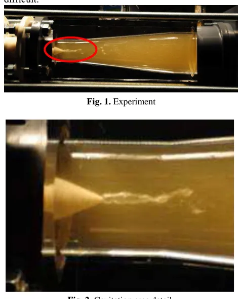
2. Experiment
University of Technology in Brno, Faculty of Mechanical Engineering, Energy Institute - Victor Kaplan Dept. of Fluid Engineering is guaranteed the experiment.
Little cavitation area is seen from the figure of the experiment (see figure 1 and figure 2), this area has the
shape of a rotating spiral. Cavitation area is too unstable and it also disappears in the experiment. Therefore, the modelling of cavitation area is very much complex and difficult.
Fig. 1. Experiment
Fig. 2. Cavitation area detail
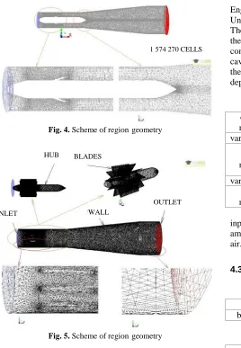
3. Geometry and grid
Investigated problem is defined as three dimensional cases (see figure 3 and figure 5). Hexahedral scheme of the grid was created in software Workbench and used for numerical simulation. The grid consists of 1574270 cells (please see). The problem was solved numerically in software Fluent 14.
Thickening on the x axis of diffuser was carried out (see figure 4), because of expected formation of a vortex rope.
Fig. 3. Scheme of region geometry INLET
BLADES
WALL HUB
Fig. 4. Scheme of region geometry
Fig. 5. Scheme of region geometry
4. Physical properties and boundary
conditions
4.1 Physical properties
Temperature of water is constant and equals 27 °C (i.e. 300 K), hence the physical model is supposed isothermal (recommended in literature). The physical properties are defined for water and vapour as constant. Water density is 998.2 kg m-3 and viscosity of water is 0.001003 Pa s. Vapour density is 0.5542 kg m-3 and viscosity of vapour is 1.34 10-5 Pa s. Air density is defined as ideal-gas and viscosity of air is 1.789 10-5 Pa s.
4.2 Boundary conditions
Variants of solutions – diffuser with generator vortices – models of cavitation:
1. Schnerr-Sauer model without air 2. Schnerr-Sauer model with air 3. Singhal model without air
4. Singhal model with air – air is defined outside the cavitation model
Boundary conditions on the inlet were defined in accordance with measured data, which were added by the Energy Institute - Victor Kaplan Dept. of Fluid
Engineering, Faculty of Mechanical Engineering, University of Technology in Brno.
The problem is solved as multiphase flow, when water is the first phase and vapour is the second one. If the air is considered in the calculation then it is defined outside the cavitation model. Due to the time dependent character of the vapour flow in cavitation region the solution is time dependent, with time step of 0.001 s.
Table 1. Boundary conditions.
outlet -
mixture outlet pressure 96525Pa variation with air
inlet - mixture
mass-flow-inlet
water 16.43996 kg s-1 vapour 1 10-8 kg s-1
air 0.000435 kg s-1 variation without air
inlet - mixture
mass-flow-inlet
water 16.4404 kg s-1 vapour 0 kg s-1 Minimum of vapour is appropriate to include the input for variant with air, it is recommended manual. The amount of water at the inlet is affected by the amount of air.
4.3 Cavitation model
Table 2. Cavitation conditions – Schnerr-Sauer model.
vaporization pressure 3500 Pa bubble number density 1013
Table 3. Cavitation conditions – Singhal model.
saturated vapour pressure 3500 Pa surface tension coefficient 0.0717 N m-1 non-condensable gas mass
fraction 2.65 10 -8
5. Numerical results
From the first series of images is apparent that cavitation region disappears gradually in a calculation. Figures 6, 7, 8 (variant A) are calculated at one time. Figures 9, 10, 11 (variant B) are calculated in a different time. It follows that the cavitation region is unstable and disappears also in the calculation.
Fig. 6. Pressure (2320 – 205707) Pa, Schnerr - Sauer model without air (variant A)
1 574 270 CELLS
INLET
HUB BLADES
WALL
OUTLET
2.06 105
1.55 105
1.04 105
5.32 104
Fig. 7. Volume fraction of vapour (0 – 0.895), Schnerr - Sauer model without air (variant A)
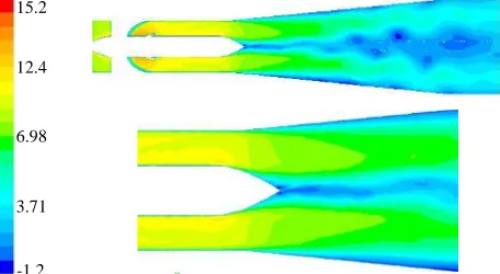
Fig. 8. X-velocity (-12.272 – 11.692) m s-1, Schnerr - Sauer model without air (variant A)
Fig. 9. Pressure (41349 – 166539) Pa, Schnerr - Sauer model without air (variant B)
Fig. 10. Volume fraction of vapour (0), Schnerr - Sauer model without air (variant B)
The results presented using Schnerr Sauer cavitation model has also described the disappearance of cavitation region.
Compared to Singhal cavitation model can be said that with increasing minimum pressure decreases the volume fraction vapour and air.
Fig. 11. X-velocity (-1.835 – 12.099) m s-1, Schnerr - Sauer model without air (variant B)
Fig. 12. Pressure (6556 – 167263) Pa, Schnerr-Sauer model with air
Fig. 13. Volume fraction of vapour + air (0 – 0,257), Schnerr-Sauer model with air
Fig. 14. X-velocity (-1,197 – 15,151) m s-1, Schnerr-Sauer model with air
0.761
0.492
0.224
0.0 0.895
6.90
0.91
-6.28
-12.3 11.7
1.41 105
1.04 105
7.25 104
4.12 104
1.66 105
9.31
5.31
0.95
-1.84 12.1
1.35 105
8.69 104
4.67 104
6.56 103
1.67 105
0.206
0.142
0.077
0.0 0.257
12.4
6.98
3.71
Singhalův cavitation model solved without air does not have comparable results with the experiment. The results indicate that there is no swirl only in the extension part (diffuser), but also by generator of vortex. But that was not the subject of a solution.
Fig. 15. Pressure (2558 – 224062) Pa, Singhal model without air
Fig. 16. Volume fraction of vapour (0 – 1), Singhal model without air
Fig. 17. X-velocity (-3.024 – 17.278) m s-1, Singhal model without air
Singhal model is suitable for solving cavitation. The presented results describe the already disappearing cavitation region (see figure 15).
The advantage of entering input of air cavitation model is that the air can then evaluated. I can also to evaluate the volume fraction of vapour and volume fraction air at the same time. It is then comparable with the experiment.
From Figure 17 is apparent that the velocity in the x direction (axis of diffuser) is negative in the cavitation area. Velocity is also negative in the swirl and generator of vortex.
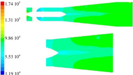
Fig. 18. Pressure (11912 – 174448) Pa, Singhal model with air
Fig. 19. Volume fraction of vapour + air (0 – 0.207), Singhal model with air
Fig. 20. X-velocity (-2.493 – 15.182) m s-1, Singhal model with air
6. Evaluation and conclusion
The aim was to map the processes of dynamic changes in cavitation, especially the shape and size of the cavitation area depending on the time.
Singhal cavitation model was chosen based on previous good experiences in the modelling of cavitation in Laval nozzle [3, 6]. Opportunity to compare the size of area of cavitation vapour at modelling in Ansys Fluent and experiment was in this task [5, 6].
Every one of calculations didn't converge. From the first variant is evident, that it depends on the time of ending the calculation. To the termination of the calculation is necessary monitoring of the mass flow on the inlet and outlet. The difference of the mass flow should be minimal. It is fulfilled in all the variants. From the first variant results verifications the hypothesis, that 1.80 105
1.13 105
4.69 104
2.56 103
2.24 105
0.75
0.50
0.25
0.0 1.0
13.2
7.13
2.05
-3.020 17.3
1.31 105
9.86 104
5.53 104
1.19 104
1.74 105
0.166
0.103
0.052
0.0 0.207
12.5
7.23
2.81
the conditions of tested variant are on the critical stability area of cavitation vortex. The cavitations vanish gradually at the experiment also the simulation result.
Schnerr Sauer cavitations model was calculate by reason of the simple definition of the cavitations conditions. Number of the bubbles is accepted in default value. Manual recommends for the solving of the cavitations use this model for its better stability.
In article are compare variants with air and without air. It is assumed, that the dissolved air is included in the water. The air volume in water at the experiment however is not exactly know.
The advantage of the setup of the air out cavitations model is possible evaluate air results, as sum of the volume fraction of air and vapour. Also from experiment it is impossible evaluate, if visible as air or vapour. Therefore sum of the volume fraction air and vapour is after it comparable with experiment.
The boundary conditions are defined for all variants identical, in accordance with measured data, which were added by the Energy Institute - Victor Kaplan Department of Fluid Engineering, Faculty of Mechanical Engineering, University of Technology in Brno.
Cavitations region in calculation is possible wrong record by reason of its unstability. It is impossible tell, that the some of the results is wrong, since cavitations region vanish also at experiment. To simpler comparing of the result is advisable to measure of the pressure values on inlet and outlet and also velocity profile on inlet areas. It would be defined exact of the boundary conditions.
References
1. M. Kozubková, Modelování proudění tekutin FLUENT, CFX. Ostrava,154 (2008)
2. M. Kozubková, Numerické modelování proudění – FLUENT I. Ostrava, (2005)
3. P. Rudolf, V. Habán, F. Pochylý, J. Koutník, K. Krüger, 52, No. 6, 109-118 (2007)
4. M. S. Plesset, R. B. Champman, 47, 283-290 (1971) 5. M. Kozubková, J. Rautová, Proceedings of the 3rd
IAHR, Brno, 583 – 592 (2009)
6. M. Kozubková, J. Rautová, M. Bojko, 39 (2012) , 7. A. K. Singhal, H. Y. LI, M. M. ATHAVALE, Y.
JIANG, ASME FEDSM'01. New Orleans, Louisiana, 2001.
8. G. H. SCHNERR, J. Sauer, Fourth International Conference on Multiphase Flow, New Orleans, 2001.
9. Ansys Fluent Inc Fluent 12.16– User’s guide. [Online]. c2009. Dostupné z: <URL:http://sp1.vsb.cz/DOC/Fluent_6.1/html/ug/ /main_pre.htm>.
Acknowledgements
The paper has been supported by project GACR 101/09/1715 „Cavitating Vortical Structures Induced by Rotation of Liquid.