Image Source Method Based Acoustic Simulation
For 3-D Room Environment
R. A. Rathnayake, W. K. I. L. Wanniarachchi
Abstract: Room Acoustics (also known as Architectural Acoustics or Building Acoustics) involves the scientific understanding of how to achieve a good sound quality within a building. The main purpose of this paper is to build a Room Acoustics Simulation which is capable to: demonstrate visualization of sound propagation around 3-D virtual room environment, examine the Room Impulse Response (RIR) and perform a less computational cost audio demonstration to understand the behavior of reverberation and echo effect. Furthermore, this paper proposes a new method to obtain the RIR for a given receiver point. In this paper, Image-Source Method (ISM) use as a modeling method for this acoustic simulation. Since all the previous works about ISM are done for 2-D room environments, this paper could be the first to implement ISM for 3-D virtual room environment.
Index Terms: Room Acoustics, Image-Source Method, Room Acoustics Simulation, 3-D virtual room environment, Room Impulse Response —————————— ——————————
1.
INTRODUCTION
Research on acoustics has been done for many decades. Acoustics is a branch of physics which tries to explain why a particular environment has good or bad acoustic qualities. There are several major branches of acoustics, among them, Room Acoustics is a vital division of the design of auditorium, theater, classroom, opera hall and etc. Room Acoustics is involved with the structural properties of a building or room, such as geometry and material properties, and the affect of these properties on the propagation of sound inside the room. With the rapid development of computer technology, now it is possible to simulate the acoustics of a room, artificially in virtual room environments, instead of doing extensive measurements, which are obviously not possible in actual real rooms. This simulation data can be used to improve the room for a given acoustic usage even before it is built.
Nowadays several different room acoustics modeling techniques have been introduced to predict acoustical characteristics of particular environments. Different modeling methods have different computational requirements and characteristics. The acoustics modeling techniques are basically divided into two main categories: wave-based methods and geometric methods. Main approaches of wave-based modeling methods are established on solving the wave equation numerically. Finite-difference time-domain (FDTD), finite-element method (FEM) and boundary element (BEM) methods are the most common techniques in this category [1]. All these wave-based modeling methods are able to provide the most accurate results. However, they are limited to low frequencies and small room environments, because these methods represent the sound wave as a group of particles. In other hands, Geometric Acoustics (GA) methods neglect all the wave properties of sound, and sound waves are considered to spread as rays [2]. This assumptions of GA methods are valid at mid and high frequencies. There are two main geometrical methods, i.e. the Ray-Tracing Method and the Image-Source Method. Among them, Image-Source Method (ISM) is proven to be the most popular one which is
very accurate and guaranteed to find all the reflection paths up to a given order or giver reverberation time [3]. This work mainly focused on building Room Acoustics Simulation for the 3-D environment. The ISM technique is used as a modeling method of the simulation. Comparing to the previous works about ISM, this paper could be the first to implement ISM for 3-D virtual room environment. Utilizing the ISM, this simulation is capable of providing,
1. Room Impulse Response (RIR) graph
2. 3-D visualization of sound propagation in a room 3. Small audio demonstration to understand the
behavior of reverberation and echo effects throughout the room.
Moreover, an alternative method to obtain the RIR graph has been introduced in this paper and this will be discussed in more detail in Section 2.3.
2
TERMS
AND
PARAMETERS
2.1 Image-Source Method
Image-Source Method (ISM) is one of Geometric Acoustic (GA) modeling method which is considered as a universal tool in many fields of acoustical and engineering research. This method has been implemented as a basic principle for a wide range of purposes including, prediction of sound propagation in indoor environments, sound rendering in virtual environments, binaural auralization, noise control in closed environments, virtual reality applications such as video games, etc. The ISM is based on the idea that, when a sound ray collides with a plane wall and the reflected sound ray can be imagined as originating from an "image-source" which is the mirror image of the original sound source created by the wall. The foundation of the image-source technique was first developed in 1899 by Carslaw [4]. In 1972, Jones & Gibbs [5] were the first to use a third-generation computer to implement the ISM to determine the sound pressure levels (SPL) in a rectangular 2D room. In 1979, Allen and Berkley published a landmark paper [6], which contained a well-established algorithm based on ISM to generate RIR in a given room environment. There are assumptions that need to be considered when using ISM. One assumption is, the sound waves (pressure waves) are replaced by the concept of sound rays which describing the path of the traveling sound energy ————————————————
R. A. Rathnayake, Department of Physics, Faculty of Applied Sciences, University of Sri Jayewardenepura, Sri Lanka. E-mail: [email protected]
223 implies that the ISM is mostly valid for high frequencies.
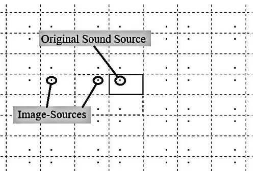
However, in 2014, Aretz and team demonstrated that the ISM grants more accurate results even at low frequencies [9]. The responsibility of the ISM is to find the pathways of all sound rays connecting the sound source and the receiver. This can be done by applying the image-source solutions to the sound source. In practice, this means that an original sound source generates mirror images of sound source against all walls in a model, thus resulting in a set of first-order image-sources. N number of surfaces will create N possible 1st order image-sources. And again, these 1st order image-sources are reflected against all the virtual-walls. This mirroring process leading to first-order, second-order and likewise up to nth-order image-sources and resulting in a lattice of image-sources, as illustrated in Fig. 1. In a way, an approximate number of possible image-sources (IS) up to the ith-order reflections, can be found using the Eq. 1. Where N is the number of surfaces.
(1)
However, the values determined using this Eq. 1 might be slightly different from the actual numbers.
Each one of image-source represents one reflection path. Fig. 2 shows that 1st order image-sources are responsible for 1st order reflection paths, 2nd order image-sources are responsible for 2nd order reflection paths and so on nth order image-sources are responsible for nth order reflection paths. The actual distance of the reflected route inside the room is exactly equal to the distance between the image source and the receiver. Considering the rectangular-shaped 2-D room with 4 walls, the ISM requires 4 first-order image-sources and 8 second-order image-sources to find all the reflection paths up to 2nd-order. The similar 3-D case would contain 6 first-order image-sources and 18 second-first-order image-sources.
2.2 Reverberation and Echo
In a closed environment like room or theater, a created sound wave will reflect by the walls multiple times until it decays due to the absorptions by the walls or objects in the space. If this reflected sound waves touched a persons’ ear in less than 0.1 seconds after the original sound wave, that person feels the effect called reverberation [10]. Since the human brain can remember the original sound wave for 0.1 seconds, there’s no time delay between the notion of the reflected wave (which came in less than 0.1 seconds) and the original wave. Therefore, the reverberation effect feels like adding fullness to the original sound wave. On the other hand, An echo effect can be heard only when the reflected sound wave takes more than 0.1 seconds to return [10]. Therefore, this reflected wave (called an echo) is clearly noticeable to the human brain and heard as a clear replica of the original sound wave. Usually, echo waves are slightly fainter than the original wave due to the energy lost as the wave travel longer distance. Usually, the reverberation effect can be heard in a closed environment and echo effect can be heard both within open and closed environments. Environments like theaters, auditoriums use reverberation effect to experience the enhanced music quality. Also some environments like lecture halls, recording studios use sound absorbing materials to control the reverberation and echo effect.
2.3 Room Impulse Response
When determining the acoustic quality of a room we have to consider the characteristic feature which is called the Room Impulse Response (RIR). The impulse response contains unit pulses (see Figure 3), which include the direct sound signal and the sound reflected by the room boundaries back to the listener. Acoustical engineers typically follow this RIR graphs to get the better idea about echo effect, distribution of late reverberations and the time delay of the signal.
Fig. 1. Lattice of image-sources (2-D view). The room is shown by a solid line box and virtual-walls are formed by thick dashed lines.
Instead of using the traditional RIR algorithms [6], this paper introduced a different method to obtain the RIR graphs with the help of ISM technique and the concept of Sound Pressure Level (SPL). Sound pressure describes pressure variations between average atmospheric pressure and the pressure in the sound wave. Sound pressure and sound volume are two entirely different things and the human ear hears only sound pressure. As shown in Eq. 2, if the distance (r) from sound-source increases, then the sound pressure (p) decreases proportionally to 1/r.
𝑝 𝑟 ∝ (2)
Human ear can detect a wide range of pressure variations. Sound Pressure Level (SPL) is a logarithmic expression, measured in decibels (dB), which is introduced to measure sound level in a particular environment. The following equation applies:
𝐿 = 0 log (
) = 20 log ( ) (3)
Where p is the effective pressure of a sound and pref is a reference sound pressure. According to the standard ANSI S1.1-1994 [11], reference sound pressure frequently identified as 20μPa in the air, which is nearly the threshold of human hearing. On the SPL scale, a sound pressure of 20μPa is 0dB, normal conversation in a room is 60dB and the loudest human voice rated at 135dB. As expressed in Eq. 2, sound pressure decreases in inverse proportion to the distance. Therefore, the sound pressure level of a spherical wavefront, which emitted by monopole sound source, decreases by -6dB each time with doubling of distance.Using Eq. 2 and 3, an expression for the sound pressure level difference (SPL attenuation; ΔL) between sound source and receiver, can be obtained as,
𝐿 = |20 log ( )| (4)
Where, ΔL – inter-zone SPL attenuation, r1 – reference distance from the sound source (usually 1m; this will be further discussed in Section IV-B) and r2 – traveling distance of sound ray. Now, Eq. 5 shows another way to find the SPL attenuation.
𝐿 = 𝐿 𝐿 (5)
Where, L1 is SPL at the point which is a reference distance (r1)
Using Eq. 6, sound pressure level at the receiver’s point (L2) can be obtained, if (L1), (r1) and (r2) values are known. In this paper, we use Eq. 6 to obtain the RIR graph. In the shoebox-shaped room environment, the receiver picks up multiple sound impulses due to the sound reflections by the walls. Moreover, each one of these reflected sound pulses comes to the receiver with a delay time, which is what causes the reverberation and echo effect. In this work, the room impulse response introduced as a time-domain plot of sound-pressure-level(dB) vs. time(s). The x-axis (time axis) of the plot indicates the delay times of direct wave and each reflection paths. The y-axis (decibel axis) of the plot will scale the sound pressure level of each path at the receiver point. The sound pressure level (L2) of direct and each reflection paths (at the receiver point) can be obtained using Eq. 6. Traveling distance (r2) and the delay time of each path can be easily found using ISM technique.
3 SYSTEM
ORGANIZATION
Fig. 3. Typical RIR graph.
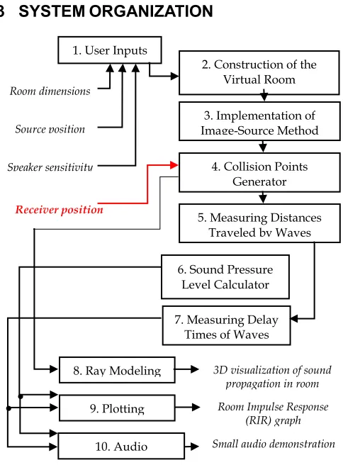
2. Construction of the Virtual Room Environment 3. Implementation of Image-Source Method
4. Collision Points Generator
5. Measuring Distances Traveled by Waves
6. Sound Pressure Level Calculator
7. Measuring Delay Times of Waves
8. Ray Modeling
9. Plotting
10. Audio Processing
Room dimensions
Source position
Speaker sensitivity
Receiver position 1. User Inputs
3D visualization of sound propagation in room
Room Impulse Response (RIR) graph
Small audio demonstration
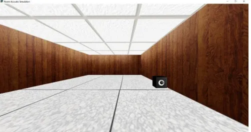
225 Fig. 5. OpenGL visualization of 3-D room environment
and audio-source (speaker).
Fig. 6. Image-Source formation (3-D view). The room is shown by a colored box. Green dot - sound source location, Blue dots - 1st order image-sources, Red dots - 2nd order image-sources. We partition our system into 10 phases (see Fig 4). Initially, for
phase 1, our simulation allows a user to input: 1) room dimensions (width, length, height); to generate virtual room environment, 2) audio source (speaker) location; to create omnidirectional virtual speaker, and 3) speaker sensitivity (this will be further discussed in Section IV-B). After getting these inputs, the simulation itself execute phase 2 and 3. Phase 2 execute in real time as a user spectate and moving through a virtual room environment. The simulation will execute phase 4 to 10 when user confirms his position as a receiver location (this will be further discussed in Section IV). Phase 8, 9 and 10 deliver result outputs of simulation.
3.1 Construction of the Virtual Room Environment
This simulation was built using Python programming language. To visualize the virtual room environment, we needed an API for rendering graphics. In the case of a Python application, such visualization tools must be implemented with separate libraries. Therefore, our potential choice, for rendering 3-D graphics, is OpenGL via Pyglet, which is open-source Python binding to OpenGL [12]. Also, our simulation uses OpenGL 3-D coordinate system to locate the position of objects, such as audio-source location, receiver location, the coordinate of every image source, etc. OpenGL has a right-handed coordinate system, with positive X-axis points right, positive Z-axis points outward the screen and positive Y-Z-axis points up [13].
Fig. 5 shows our virtual room environment, which was built upon the room dimensions that input by the user. In addition, a small speaker is created in the room, depending on the ‘audio-source location’ input. In here, user can spectate the room in first person view and simulation allow the user to free roam around the room environment using W, A, S, D keys.
3.2 Implementation of Image-Source Method
Now, after generating the virtual environment, the simulation itself run an algorithm called ‘IS Generator’(phase 3) to create image sources. This image source generating algorithm capable of creating image sources around the room environment by mirroring audio-source location coordinate. This system was programmed to create image sources up to
2nd-order. Therefore, our simulation is capable of showing all the
paths of the reflections of sound waves up to 2nd-order. Figure 6 illustrates a quick example of image-source formation in 3-D space. Since, our simulation limits image sources up to 2nd-order, image source generating algorithm create 6 first-order image-sources and 18 second-order image-sources. All the 6 of first-order image-sources are mirror images of original audio-source (speaker). And other 18 of second-order image-audio-sources are mirror images of first-order image-sources. This mirroring process has been discussed in detail in Section II-A. Therefore, each one of first-order image-sources will be responsible for 1st-order reflections and second-1st-order image-sources will responsible for 2nd-order reflections. Position coordinates of every image-source will be remembered by the simulation for further calculations and result outputs.
4 RESULTS
AND
SIMULATION
End-user can obtain 3 results from this simulation. Before obtaining results, user has to lock his position as ‘receiver’ point. Earlier mentioned that in this simulation user allowed to spectate and move around the virtual room. When user pressed ‘L’ key, while standing in whatever position he wants in the room, system takes his current position as a receiver (listener). In this way, a user can select ‘receiver’ location as desired. Now, this receiver location coordinate is used by several algorithms to simulate results.
4.1 3D Visualization of Sound Propagation
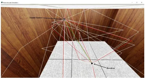
Sound waves in air are longitudinal pressure waves that exist in our physical environment. Nobody can't see them, but there are many indirect ways to visualize these waves. In this work, with the help of IMS, our simulation uses geometric rays to visualize sound propagation in our virtual 3D room environment. Therefore, a user can get a quick understanding of how sound rays propagate from the sound source (speaker) to the receiver (listener). This simulation is capable of showing direct wave, 1st-order reflection and the 2nd-order reflection of the sound rays.
Fig. 7. Propagation of sound rays (for case I). Green line - direct wave, Red lines - 1st order reflections, White lines - 2nd order reflections.
Fig. 8. Propagation of sound rays (for case II). Green line - direct wave, Red lines - 1st order reflections, White lines - 2nd order reflections.
Fig. 9. Propagation of sound rays (for case III). Green line - direct wave, Red lines - 1st order reflections, White lines - 2nd order reflections.
This Collision Points Generator algorithm is mainly responsible for 2 tasks: 1) determining which image-source is responsible for each reflection path, 2) calculating and sending the
coordinates of every point of collisions (done by each
reflection path) on the wall. Ray Modeling function need all these coordinates: 1) audio-source point, 2) wall-collision points, 3) receiver point, to draw the direct wave and all the reflection paths of sound up to 2nd-order. Figures 7, 8 and 9 show some selected test runs done on the simulation. Case I: Room dimensions:- width = 7 m, height = 4 m, length = 10 m. Room type:- ‘lecture hall’. Distance from sound-source (speaker) to receiver is 4.3 m. Case II: Room dimensions:- Same as in case I. Room type:- ‘lecture hall’. Distance from sound-source to receiver is 4.96 m. Receiver location is same as in case I, but different Sound-Source location. In these cases, we created two different types of room environments: small lecture hall (Fig. 7 & 8) and large main hall (Fig. 9). To observe different results, in case I & II we kept the receiver location fixed and only changed the sound source location, and in case III, we set random receiver and sound source location. As shown in results, a user can observe direct wave (green line), 6 first-order reflection paths (red lines) and 18 second-order reflection paths (white lines). Case III: Room dimensions:- width = 20 m, height = 10 m, length = 25m. Room type:- ‘large main hall’. Distance from sound-source to
surfaces without being scattered, which means diffuse reflections almost neglected here. Usually sound waves (or light) scattered at many different angles when they incident on the rough surface. This effect is known as Diffuse Reflection
[14]. Hence, our simulation gives a very rough idea about how sound rays propagate in a particular room environment.
4.2 Room Impulse Response (RIR) Graph
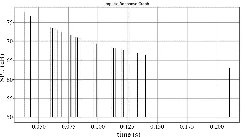
227 Fig. 10. RIR graph related to the case I.
Fig. 11. RIR graph related to the case II.
Fig. 12. RIR graph related to the case III.
Figures 10, 11 and 12 respectively show the plotted RIR results for the environmental conditions previously explained in case I, II and III. For all the cases we entered fixed speaker sensitivity value (as 90dB) to observe the different results. Each RIR graph clearly indicates the sound-pressure-levels of each sound rays that came at the receiver point. Furthermore, reverberation and echo effects can also be observed using these results. First impulse which has the highest SPL value always represent the direct wave. All the impulses up to 0.1 seconds from the time that the direct wave arrives, are known as early reverberations. The rest is a collection of late reverberations and echoes. We can get an idea about how the receiver hears early and late reverberation effect at the receiver point, by examining the Figures 10 and 11, which related to the case I and II. The last two impulses of RIR graph shown in Figure 12 clearly indicate the echo effect at the receiver point. When a sound wave collides with the specific
material part of its energy is reflected, another part is transmitted through the material and the rest is absorbed into the material [16]. This simulation was built upon neglecting these sound absorptions. Therefore, in our environment, all sound rays will reflect from all surfaces without losing any energy. Hence, in this case, we assumed that the reflections by the surfaces do not affect or reduce the sound pressure of the waves.
4.3 Audio Demonstration
Additionally, our simulation is capable of playing some audio file for short duration through our virtual speaker. Therefore, while sitting on the receiver point, a user can hear that audio clip as well as can hear the reverberations/echoes of that sound. Hence, by using our virtual environment, a user can get a deep idea about how a person hears the reverberations and echoes, at the receiver point, in the real environment. Our ‘AudioProcessing’ algorithm (see phase 10 on Fig. 4) is mainly responsible for playing, adding and mixing the audio file. This algorithm imports datasets from ‘Sound Pressure Level Calculator’(phase 6) and ‘Delay Time Calculator’(phase 7) algorithms to add the reverberation and echo effects to the audio clip
5
CONCLUSIONS
The aim of this study was to develop an image-source method-based acoustics simulation for 3-D room environment. We decided to select this ISM technique because of its higher accuracy and simplicity. As compared to previous ISM based acoustic modeling approaches, our simulation could be the first to implement ISM for 3-D virtual room environment. As for results, our simulation is able to: 1) visualize sound propagation in a 3-D virtual room, 2) deliver the RIR graph and, 3) perform a small audio demonstration to understand the behavior of reverberation and echo effects. Additionally, an alternative method to obtain the RIR graph has been proposed in this paper. In order to test the simulation, we have created three different environments, and observed results have been discussed. In this work, we encourage to use this ISM technique for 3D applications like virtual reality games. As for the future developments, we are willing to add the sound absorption coefficient into the system and, as well as expecting to upgrade the ISM up to 3rd of 4th order to obtain much more accurate results.
REFERENCES
[1] P. Svensson and U. Kristiansen, "Computational Modelling and Simulation of Acoutic Spaces", in AES 22nd Conf. on Virtual, Synthetic and Entertainment Audio, 2002, pp. 11-30.
[2] L. Savioja and U. Svensson, "Overview of geometrical room acoustic modeling techniques", The Journal of the Acoustical Society of America, vol. 138, no. 2, pp. 708-730, 2015. Available: 10.1121/1.4926438.
[3] P. Samarasinghe, T. Abhayapala, Y. Lu, H. Chen and G. Dickins, "Spherical harmonics based generalized image source method for simulating room acoustics", The Journal of the Acoustical Society of America, vol. 144, no. 3, pp. 1381-1391, 2018. Available: 10.1121/1.5053579. [4] H. Cakslaw, "Some Multiform Solutions of the Partial
10.1112/plms/s1-30.1.121.
[5] B. Gibbs and D. Jones, "A Simple Image Method for Calculating the Distribution of Sound Pressure Levels within an Enclosure", Acta Acustica united with Acustica, vol. 26, pp. 24-32, 1972.
[6] J. Allen and D. Berkley, "Image method for efficiently simulating small‐room acoustics", The Journal of the Acoustical Society of America, vol. 65, no. 4, pp. 943-950, 1979. Available: 10.1121/1.382599.
[7] M. Vorländer, Auralization. Berlin, Heidelberg: Springer-Verlag Berlin Heidelberg, 2008.
[8] J. Rindel, "The Use of Computer Modeling in Room Acoustics", Journal of Vibroengineering, vol. 3, no. 4, pp. 219-224, 2000.
[9] M. Aretz, P. Dietrich and M. Vorländer, "Application of the Mirror Source Method for Low Frequency Sound Prediction in Rectangular Rooms", Acta Acustica united with Acustica, vol. 100, no. 2, pp. 306-319, 2014. Available: 10.3813/aaa.918710.
[10]M. Wölfel and J. McDonough, Distant speech recognition. Chichester, U.K: Wiley, 2009, pp. 48-49.
[11]Acoustic Terminology, ANSI S1.1-1994, 1994.
[12]Pyglet Home - Bitbucket, Bitbucket.org. [Online]. Available: https://bitbucket.org/pyglet/pyglet/wiki/Home. [13]LearnOpenGL - Coordinate Systems, Learnopengl.com.
[Online]. Available: https://learnopengl.com/Getting-started/Coordinate-Systems.
[14]H. Nironen, "Diffuse Reflections in Room Acoustics Modelling", M. Tech. thesis, Helsinki University of Technology, Espoo, Finland, 2004.
[15]How to: Speaker Sensitivity | Klipsch, Klipsch. [Online]. Available: https://www.klipsch.com/education/speaker-sensitivity.