A flowgraph model for bladder carcinoma

R E S E A R C H

Open Access

A flowgraph model for bladder carcinoma

Gregorio Rubio

, Belén García-Mora

, Cristina Santamaría

, José Luis Pontones

From

1st International Work-Conference on Bioinformatics and Biomedical Engineering-IWBBIO 2013

Granada, Spain. 18-20 March 2013

* Correspondence: grubio@imm. upv.es

1_{Instituto de Matemática}

Multidisciplinar, Universitat Politècnica de València, España

Abstract

Background:Superficial bladder cancer has been the subject of numerous studies for many years, but the evolution of the disease still remains not well understood. After the tumor has been surgically removed, it may reappear at a similar level of malignancy or progress to a higher level. The process may be reasonably modeled by means of a Markov process. However, in order to more completely model the evolution of the disease, this approach is insufficient. The semi-Markov framework allows a more realistic approach, but calculations become frequently intractable. In this context, flowgraph models provide an efficient approach to successfully manage the evolution of superficial bladder carcinoma. Our aim is to test this methodology in this particular case.

Results:We have built a successful model for a simple but representative case. Conclusion:The flowgraph approach is suitable for modeling of superficial bladder cancer.

Background

Bladder tumors are a challenge in urology. They pose an important public health pro-blem because they are biologically very aggressive and are highly prevalent in western countries. Approximately 75-85 % of patients with newly diagnosed bladder carcinoma have non muscle-invasive bladder carcinoma (NMI-BC), which can be managed with transurethral resection (TUR). TUR is a surgical endoscope technique used to remove the macroscopic tumor from the interior of the bladder. However it has a notable tendency to recur (30-85 %) and less frequently to progress to muscle invasive stages (10-20 %). The object of this study is the NMI-BC, that makes up 70 % of the total health care cost of this disease. A review about the NMI-BC may be found in [1].

Biotechnological advances have allowed us to use different therapeutic procedures (surgery, radiotherapy, chemotherapy, immunotherapy) successfully but still many patients suffer an unfavourable outcome without control of disease. In practice urolo-gists have a serious problem: some patients with similar characteristics undergo differ-ent evolution. Consequdiffer-ently, this creates a problem as to the choice of treatmdiffer-ent to be applied. Urologists need tools to accurately predict the real evolution of the disease, that help them to improve treatment modalities and follow-up schemes of non-muscle invasive bladder cancer patients. In this regard an important contribution [2] appeared in European Urology, the official journal of the European Association of Urology.

By means of looking up tables the probability of recurrence and progression for a patient is provided. However only time to first recurrence is considered, and the analy-sis is reduced to the Cox proportional hazards regression model. Later works have stu-died the model validation, finding some limitations [3].

Our team has been working with urologists from University Hospital La Fe for the last ten years. We have developed several models trying to capture different aspects of the disease evolution. Our aim for the near future is to detect the most relevant predictive factors, and also to perform an accurate model of the disease evolution. The first objec-tive includes investigating at the genetic and molecular level, while the second one could be achieved with a suitable multistate model. While the process may be reasonably mod-eled by means of a Markov process, in order to more completely model the evolution of the disease this approach is insufficient. Specifically, it is possible that time spent in a state influences the future evolution of the process, i.e., it not only depends on the cur-rent state. The semi-Markov framework allows a more realistic approach, but calcula-tions become frequently intractable. In this context, flowgraph models provide an efficient approach for the analysis of time-to-event data, since their introduction in this field a few years ago [4]. The present work is a first step in order to explore the evolution of the recurrence progression process by means of this methodology.

The paper is organized as follows: first we review a few basic concepts of survival analysis, phase-type distributions and Erlang distributions, needed to build the model. Then we present the essentials of flowgraph models and important features of our approach. The section that follows deals with a simple flowgraph model for the recur-rence-progression process in NMI-BC, constructed using a database from La Fe University Hospital of Valencia (Spain). Finally, some conclusions are discussed.

Survival analysis and phase-type distributions Survival analysis

Survival analysis techniques deal with the analysis of data taking times from a well-definedtime-origin until the occurrence of some particular event orend-point.

To summarize survival data there are two key functions: the Survival Function and the Hazard Function. Let T be the random variable associated with the survival time (time until the ocurrence of the event).

The Survival Function is

S(t) = P(T≥ t) = 1−F(t)

where F(t) is the distribution function of T. It expresses the probability that an indi-vidual survives from the time origin to some time beyondt.

The Hazard Function is given by

λ(t) = lim t→0

P(t≤T<t+t|T≥t)

t ,

which expresses the hazard rate or the instantaneous event rate.

434 underwent a recurrence, 24 a progression, and 499 had censored times, which means that at the time of their last check-up they had no recurrence or progression.

Phase-type distributions

In order to model lifetimes, mixtures of distribution functions are useful. In this con-text phase-type distributions [6] are very interesting, because of their properties and they provide computations with manageable analytical expressions. Let us summarize the main concepts: the distribution F(-) on [0,∞) is a phase-type distribution (PH-distribution) with representation (a, T) if it is the distribution of the time until absorp-tion in a Markov process on the states {1, . . . ,m, m+ 1} with generator

T T0

0 0

,

and initial probability vector (a,am+1) whereais a row m-vector.

The matrix T of order mis singular with negative diagonal entries and non-negative off-diagonal entries, T0 is a column matrix with nonnegative entries, and it holds that

−Te=T0,

whereedenotes a column vector with all components equal to one. The distributionF(-) is given by

F(t) = 1−αexp(Tt)e, t≥0 (1)

and the density f(t) by

f(t) =αexp(Tt)T0.

The survival function is

S(t) =αexp(Tt)e (2)

and the hazard function is given by

h(t) = αexp(Tt)T 0

αexp(Tt)e .

Finally, the Laplace transform is

L(s) =αm+1+α(sI−T)−1T0, for Re(s)>0. (3) Phase-type distributions are a closed class for finite mixtures, and form a class weakly dense in the class of general distributions defined on the positive real line.

A particular case of phase-type distribution, relevant in our approach, is the Erlang dis-tribution. An Erlang distributionE[r,l] has a representation (a, T) as a phase-type [7]:

α= (1, 0,. . ., 0)1×r

T= ⎛ ⎜ ⎜ ⎜ ⎜ ⎜ ⎝ −λ λ −λ λ . .. ... −λ λ −λ ⎞ ⎟ ⎟ ⎟ ⎟ ⎟ ⎠

A finite mixture of Erlangs distributions is therefore a phase-type distribution. We are interested in the class of mixtures of three Erlang distributions studied in [8]. The distribution function of the elements in this class is given by the expression

G(t) =p1F1(t) +p2F2(t) +p3F3(t), (4)

withp1+p2+p3 = 1,pi> 0,i = 1, 2, 3.

Let us denote the three Erlangs by E[r1, µ1], E[r1, µ1],E[r1,µ1], with µi> 0 andri a

positive integer,i= 1, 2, 3. In the particular case with r1 = 1,r2= 3, r3 = 5 the repre-sentation as phase-type distribution is (a, T) where

α= (p1 p2 0 0 p3 0 0 0 0) (5)

T= ⎛ ⎜ ⎜ ⎜ ⎜ ⎜ ⎜ ⎜ ⎜ ⎜ ⎜ ⎜ ⎜ ⎝

−μ1 0 0 0 0 0 0 0 0

0 −μ2 μ2 0 0 0 0 0 0

0 0 −μ2 μ2 0 0 0 0 0

0 0 0 −μ2 0 0 0 0 0

0 0 0 0 −μ3 μ3 0 0 0

0 0 0 0 0 −μ3 μ3 0 0

0 0 0 0 0 0 −μ3 μ3 0

0 0 0 0 0 0 0 −μ3 μ3

0 0 0 0 0 0 0 0 −μ3

⎞ ⎟ ⎟ ⎟ ⎟ ⎟ ⎟ ⎟ ⎟ ⎟ ⎟ ⎟ ⎟ ⎠ (6)

The versatility of distributions given in (4) let have us several options to fit them to our interest distributions. The way we tried was to perform some experimental compu-tations, considering different values of r1,r2andr3. Mixture (5) was explicitly given in [8], and we found it worked very well.

Flowgraph models

A flowgraph model is a graphical representation of a multistate model that consists of directed line segments (branches) connecting the states, namely, a directed graph. The branches are labeled with transmittances, that are the transition probability pij from

statei to statejmultiplied by an integral transformGij(s) of the transition time

prob-ability density function (PDF). This transformation can be a characteristic function (CF), a moment generating function (MGF), a Laplace transform (LT), or even an empirical transform [9][10]. Flowgraphs are used to represent semi-Markov processes, given that allowed waiting time distributions go beyond the exponential distribution directly linked to Markov processes.

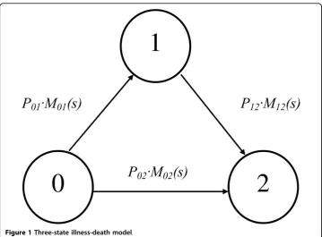
For instance, Figure 1 shows the flowgraph of the three-state illness-death model that we will use in this paper, based on [11].

Transmittances are combined according to a systematic procedure (see [12], section 2.5), in order to compute the transforms for the transitions of interest. For instance, the rules pertaining to the graph in the Figure 1 are the following:

1) The transmittance of transitions in series is the product of the series transmittances.

2) The transmittance of transitions in parallel is the sum of the parallel transmittances.

In order to perform the model, the first step is to select a suitable distribution for the waiting time in each transition. Our approach will be to compute the empirical dis-tributions (Kaplan-Meier [5]) and approximate them using mixtures of Erlang distribu-tions. Specifically we use the mixture given by (5)-(6). Note that the cumulative distribution function is easily computed from expression (1). The parameters piandµi

are calculated by minimizing

||Fij(t)−Gij(t)||, (7)

where Fij is the empirical distribution for the transition ij andGijthe mixture

distri-bution for the same transition. Initial values for the minimization process are needed. In order to estimate these values (and also to decide a suitable mixture, in our case (5)-(6)) we use a non-negative least squares fit (Lawson-Hanson algorithm [13]).

More precisely, the idea is the following. Based on [8], we try several Erlang distribu-tions in expression (4). Given F1,F2 andF3, and an empirical distribution Fwe con-sider the system

F=p1F1+p2F2+p3F3 1 =p1+p2+p3

which we fit by non-negative least squares, to compute p1,p2 andp3. In this way we obtain reasonable initial values for the parameters piand µi.

Once the parametric distributions have been computed, the Laplace transforms are easily calculated from (3). Then we compute the Laplace transform relevant to the transitions of interest, applying the above rules. The final step is to invert these trans-forms to obtain PDFs, for which we use an inversion algorithm called EULER, devel-oped by Abate and Whitt [14].

Flowgraph models for stochastic networks were introduced by Butler and Huzurba-zar [4]. An account of the theory developed up to 2005 may be found in [12]. A recent contribution proposing a prognostic model is [15].

A flowgraph model for bladder carcinoma Data

The database was obtained from La Fe University Hospital of Valencia (Spain). It records clinical-pathological information from 957 patients, followed between January 1995 and January 2010. The primary tumor is a NMI-BC, which means that it is cate-gorized as stage Ta or T1, according to the World Health Organization (WHO) TNM classification staging system [16]. After removal of the tumor by TUR, it may recur at a similar stage, which we call recurrence; or it may progress to muscle invasive stages T2, T3 or T4, which we call progression. The data record several recurrence times. This means that some patients have no recurrence at all, some have one or more recurrences, and some have progression (directly of after some recurrence). In our model we have considered progression and one recurrence. As stated above, 434 patients underwent a recurrence, 24 a progression, and 499 had censored times. Then, 63 patients were lost. From the remaining 371 patients, 17 underwent a progression, 226 a recurrence and times of the remaining 128 patients were censored. A full description of data may be found in [17].

Flowgraph model

Our aim in this paper is to test the flowgraph methodology in this particular problem, and so we perform the simple model of Figure 1. In state 0 the patient is free of dis-ease, after the TUR of the primary tumor. State 1 is the first recurrence, and state 2 is progression. Time is given in years.

By way of example, we are going to model the overall risk of progression. So we are interested in finding the probability distribution of time to reach state 2 for the first time starting in state 0, irrespective of the path that was taken. That is to say, the first passage distribution of going from disease free to muscle invasive stages. But the aim of a more general flowgraph model for the recurrence - progression process would be to predict the risk of recurrence or progression from any state.

Parametric distributions for all transitions and their Laplace transforms are per-formed according to the procedure described above. Minimization is carried out by means of the constrOptimfunction, from the R Stats Package [18]. We use the eucli-dean norm in (7). Empirical and parametric distributions for each transition are shown in Figures 2, 3 and 4.

Let us calculate the first passage distribution of going from state 0 to state 2. For this we compute the Laplace transform of the time to progression. Applying the rules 1 and 2 above, it would be given by:

LT(s) =p01p12LT01(s)LT12(s) +p02LT02(s)

Figure 2Erlang mixture (smooth line) and empirical distribution (step function) for transition 01.

divide the precedingLT(s) by this probability to obtain the true Laplace transform [12, pag. 19]

LT(s) = p01p12LT01(s)LT12(s) +p02LT02(s)

p01p12+p02

Figure 4Erlang mixture (smooth line) and empirical distribution (step function) for transition 12.

Probabilities pijare assigned from estimations based on our data. They simply consist

of the ratios between the number of progressions or recurrences and the number of patients who could undergo the relevant transition. Calculations are quite sensitive to these values. We tried with the current and also previous database. The best results were obtained takingp01= 0.3967742,p02= 0.02507837 andp12= 0.03252033.

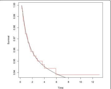
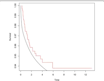
To recover the PDF we use a variant of the inversion algorithm EULER [15]. From this function we obtain the survival function (with regard to progression), that is shown in Figure 6, jointly with the empirical survival function. The hazard function may be also easily computed. Thus we have a parametric model to predict the prob-ability of being free of progression at a given time. The procedure may be easily used to define risk groups, simply by calculating the survival functions of patients grouped according to common characteristics. Then the monitoring and treatment of patients can be adjusted according to their risk.

All computations were made in R. Besides the mentioned packages, we also used the expm [19], Matrix [20] and survival [21] packages.

Discussion

A parametric approach in the framework of flowgraph models involves exploring para-metric models looking for the distributions that match the data better. In [12] histo-grams of sample waiting times are suggested. In this paper we propose a fitting procedure using mixture of Erlang distributions. Figures 2, 3 and 4 show graphically that the fitted parametric distributions match the empirical distributions very well.

Figure 6 shows that parametric distribution provided by the model matches also the empirical distribution of our interest transition very well.

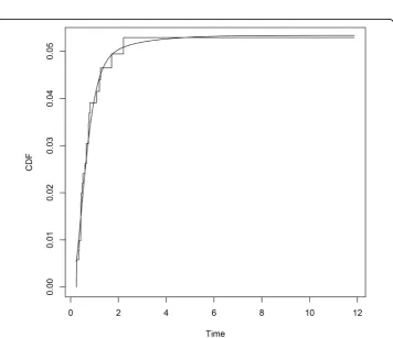
In order to contrast our results with other approaches, we have performed the classical multistate Markov model. The msm R package by C. Jackson [22] is a useful tool to man-age Multi-state Markov and hidden Markov models in continuous time. Using this soft-ware, we found some similarities with our results, but overall they were worse, probably because the Markovian hypothesis is not satisfied. By way of example, Figure 7 corre-sponds to the first passage distribution of going from state 0 to state 2.

This is only a first step in applying the flowgraph approach to bladder carcinoma. Our aim is to incorporate covariates in a parametric model involving several recur-rences and progression. Thus the doctors will have a useful tool to estimate the risk of recurrence and progression of patients according to their characteristics.

Conclusions

These results suggest that the approach is suitable for modeling the evolution of the NMI-BC. Therefore it is justified to try to extend the model to more complex situations. Flowgraph methodology is very flexible. It allows the model to incorporate multiple recurrences, and recently also covariates [9]. Moreover non-parametric approaches are also available [10]. This versatility, along with the inclusion of molecular biomarkers, allow us to expect to get a very accurate model in a not too distant future.

Competing interests

The authors declare that they have no competing interests.

Figure 7Survival function of Markov model (smooth line) and empirical survival function (step

Authors’contributions

GR, BG and CS did the work of mathematical modeling. JLP addressed the medical context and obtaining tumor samples.

Acknowledgements

This study has been funded by Vicerrectorado de Investigación de la Universitat Politècnica de València. Reference 2406. The authors thank Dave Collins for his support and specially his EULER code in R, and the two anonymous referees for many helpful comments and valuable suggestions which improved the content of the paper.

Declarations

Publication of this article has been funded by Universitat Politècnica de València (Spain).

This article has been published as part ofTheoretical Biology and Medical ModellingVolume 11 Supplement 1, 2014: Selected articles from the 1st International Work-Conference on Bioinformatics and Biomedical Engineering-IWBBIO 2013. The full contents of the supplement are available online at http://www.tbiomed.com/supplements/11/S1.

Authors_’details

1

Instituto de Matemática Multidisciplinar, Universitat Politècnica de València, España.2Departamento de Urología, Hospital Politécnico La Fe, Valencia, España.

Published: 7 May 2014

References

1. van Rhijn BW, Burger M, Lotan Y, Solsona E, Stief CG, Sylvester RJ, Witjes JA, Zlotta AR:Recurrence and progression of disease in non-muscle-invasive bladder cancer: from epidemiology to treatment strategy.Eur Urol2009,56:430-42. 2. Sylvester RJ, van der Meijden AP, Oosterlinck W, Witjes JA, Bouffioux C, Denis L, Newling DW, Kurth K:Predicting

recurrence and progression in individual patients with stage Ta T1 bladder cancer using EORTC risk tables: a combined analysis of 2596 patients from seven EORTC trials.Eur Urol2006,49:475-7.

3. Fernández-Gómez J, Madero R, Solsona E, Unda M, neiro LMP, González M, Portillo J, Ojea A, Pertusa C, Rodríguez-Molina J, Camacho J, Rabadan M, Astobieta A, Montesinos M, Isorna S, nola PM, Gimeno A, Blas M, neiro JAMP:The EORTC Tables Overestimate the Risk of Recurrence and Progression in Patients with Non-Muscle-Invasive Bladder Cancer Treated with Bacillus Calmette-Guerin: External Validation of the EORTC Risk Tables.Eur Urol2011,60:423-30.

4. Butler RW, Huzurbazar AV:Stochastic network models for survival analysis.J Am Statist Assoc1997,92:246-57. 5. Klein JP, Moeschberger ML:Suvival Analysis Techniques for Censored and Truncated Data.segunda edition. Springer; 2003. 6. Neuts MF:Matrix Geometric Solutions in Stocastic Models An Algoritmic ApproachBaltimore: The Johns Hopkins University

Press; 1981.

7. Latouche G, Ramaswami V:Introduction to Matrix Analytic Methods in Stochastic ModelingPhiladelphia: SIAM; 1999. 8. Pérez-Ocón R, Segovia MC:Modeling lifetimes using phase-type distributions.InRisk, Reliability and Societal Safety,

Proceedings of the European Safety and Reliability Conference 2007 (ESREL 2007)Taylor & Francis re 2007.

9. Huzurbazar A, Williams B:Incorporating Covariates in Flowgraph Models: Applications to Recurrent Event Data.

Thecnometrics2010,52:198-208.

10. Collins DH, Huzurbazar AV:System reliability and safety assessment using non-parametric flowgraph models.

Proceedings of the Institution of Mechanical Engineers, Part O: Journal of Risk and Reliability December 1, 2008 vol 222 no 4

2008, 667-664.

11. Huzurbazar A:Multistate Models, Flowgraph Models, and Semi-Markov Processes.Communications in Statistics -Theory and Methods2004,33:457-474.

12. Huzurbazar A:Flowgraph Models for Multistate Time-To-Event DataNew York: Wiley; 2005.

13. Mullen KM, van Stokkum IHM:nnls: The Lawson-Hanson algorithm for non-negative least squares (NNLS)2012 [http:// CRAN.R-project.org/package=nnls], [R package version 1.4].

14. Abate J, Whitt W:The Fourier-Series Method For Inverting Transforms Of Probability Distributions.Queueing Syst

1992, 5-88.

15. Collins DH, Huzurbazar AV:Prognostic models based on statistical flowgraphs.Appl Stochastic Models Bus Ind2012,

28:141-51.

16. OMS:International Classification of Tumours2_™, World Health Organization, Histological typing of urinary bladder tumours; 1999, Volumen 10, Geneva.

17. Lujan S:Modelización matemática de la multirrecidiva y heterogeneidad individual para el cálculo del riesgo biológico de recidiva y progresión del tumor vesical no músculo invasivo.PhD thesisUniversitat de València; 2012. 18. Team RDC:R: A Language and Environment for Statistical ComputingR Foundation for Statistical Computing, Vienna,

Austria; 2010 [Http://www.R-project.org].

19. Goulet V, Dutang C, Maechler M, Firth D, Shapira M, Stadelmann M, expm-developers@listsR-forgeR-projectorg:expm: Matrix exponential2011 [http://CRAN.R-project.org/package=expm], [R package version 0.98-5].

20. Bates D, Maechler M:Matrix: Sparse and Dense Matrix Classes and Methods2011 [http://CRAN.R-project.org/ package=Matrix], R package version 1.0-1.

21. Therneau T:survival: Survival analysis, including penalised likelihood2011 [http://CRAN.R-project.org/package=survival], original Splus: R port by Thomas Lumley, [R package version 2.36-10].

22. Jackson CH:Multi-State Models for Panel Data: The msm Package for R.Journal of Statistical Software2011,

38(8):1-29[http://www.jstatsoft.org/v38/i08/].

doi:10.1186/1742-4682-11-S1-S3