R E S E A R C H
Open Access
Efficient robust image interpolation and
surface properties using polynomial texture
mapping
Mingjing Zhang and Mark S Drew
*Abstract
Polynomial texture mapping (PTM) uses simple polynomial regression to interpolate and re-light image sets taken from a fixed camera but under different illumination directions. PTM is an extension of the classical photometric stereo (PST), replacing the simple Lambertian model employed by the latter with a polynomial one. The advantage and hence wide use of PTM is that it provides some effectiveness in interpolating appearance including more complex phenomena such as interreflections, specularities and shadowing. In addition, PTM provides estimates of surface properties, i.e., chromaticity, albedo and surface normals. The most accurate model to date utilizes multivariate Least Median of Squares (LMS) robust regression to generate a basic matte model, followed by radial basis function (RBF) interpolation to give accurate interpolants of appearance. However, robust multivariate modelling is slow. Here we show that the robust regression can find acceptably accurate inlier sets using a much less burdensome 1D LMS robust regression (or ‘mode-finder’). We also show that one can produce good quality appearance interpolants, plus accurate surface properties using PTM before the additional RBF stage, provided one increases the dimensionality beyond 6D and still uses robust regression. Moreover, we model luminance and chromaticity separately, with dimensions 16 and 9 respectively. It is this separation of colour channels that allows us to maintain a relatively low dimensionality for the modelling. Another observation we show here is that in contrast to current thinking, using the original idea of polynomial terms in the lighting direction outperforms the use of hemispherical harmonics (HSH) for matte appearance modelling. For the RBF stage, we use Tikhonov regularization, which makes a substantial difference in performance. The radial functions used here are Gaussians; however, to date the Gaussian dispersion width and the value of the Tikhonov parameter have been fixed. Here we show that one can extend a theorem from graphics that generates a very fast error measure for an otherwise difficult leave-one-out error analysis. Using our extension of the theorem, we can optimize on both the Gaussian width and the Tikhonov parameter.
Keywords: Polynomial texture mapping; Photometric stereo; Radial basis functions; Hemispherical harmonics; Robust regression
1 Introduction
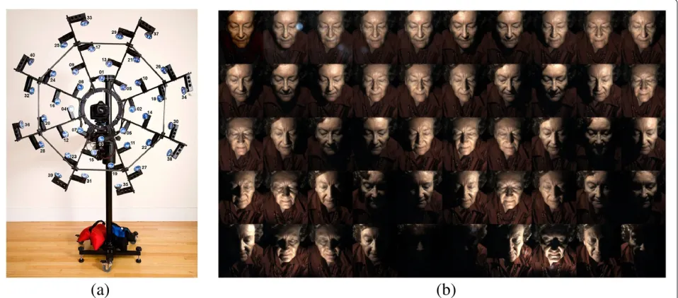
Polynomial texture mapping (PTM) [1] uses a single fixed digital camera at constant exposure, with a set of n images captured using lighting from different direc-tions. A typical rig would consist of a hemisphere of xenon flash lamps imaging an object, where directions to each light is known (Figure 1a). The basic idea in PTM is to improve on a simple Lambertian model for matte
*Correspondence: [email protected]
School of Computing Science, Simon Fraser University, Vancouver, British Columbia V5A 1S6, Canada
content, whereby the three components of the light direc-tion are mapped to luminance, by extending the model to include a low-order polynomial of lighting-direction components. The strength of PTM, in comparison to a simple Lambertian photometric stereo (PST) [2] is that PTM can better model real radiance and to some extent grasp intricate dependencies due to self-shadowing and interreflections. Usually, some 40 to 80 images are cap-tured. The better capture of details is the driving force behind the interest in this technique evinced by many museum professionals, with the original least squares
(LS)-based PTM method already in use at major museums in the USA, including the Smithsonian, the Museum of Modern Art and the Fine Arts Museums of San Francisco, and is planned for the Metropolitan and the Louvre (M. Mudge, personal communication, Cultural Heritage Imaging). As well, some work has involved applying PTM in situfor such applications as imaging palaeolithic rock art [3]. In such situations, one has to recover lighting directions from the specular patch on a reflective sphere [4]; such a ‘highlight’ method [5] can also be applied to museum capture of small objects or to microscopic image capture.
PTM generates a matte model for the surface, where luminance (or RGB) is modelled at each pixel via a polynomial regression from light-direction components to luminance. Say, e.g. there are n = 50 images, with n known normalized light-direction three-vectors a. Then in the original embodiment, a six-term polyno-mial model is fitted at each pixel separately, regressing onto that pixel’snluminance values using LS regression. The main objectives of PTM are the ability to re-light pixels using the regression parameters obtained, as well as the recovery of surface properties: surface normal, colour and albedo. For re-lighting, the idea is simply that if the regression from the n in-sample light-directions a to n luminance values, L is known then substituting a new a will generate a new L, thus yielding a sim-ple interpolation scheme for new, out-of-samsim-ple, light directionsa.
In [6], we extend PTM in three ways: First, the six-term polynomial is changed so as to allow purely linear terms to model purely linear luminance exactly. Sec-ondly, the LS regression for the underlying matte model is replaced by a robust regression, the least median of squares (LMS) method [7]. This means that only a major-ity of the n pixel values obtained at each pixel need be actually matte, with specularities and shadows automati-cally identified as outliers. With correctly identified matte pixels in hand, surface normals, albedos and pixel chro-maticity are more accurately recovered. Thirdly, authors in [6] further add an additional interpolation level by modelling the part of in-sample pixel values that is not completely explained by the matte PTM model via a radial basis function (RBF) interpolation. The RBF model does a much better job of modelling features such as spec-ularities that depend strongly on the lighting direction. As well, the RBF approach can make use of any shadow information to help model interpolated shadows, which change abruptly with lighting direction. The interpola-tion is still local to each pixel and, thus, does not attempt to bridge non-specular locales as in reflectance sharing, for example [8,9]. In reflectance sharing, aknownsurface geometry is assumed, as opposed to the present paper. Here, we rely on the idea that there is at least a small
contribution to specularity at any pixel, e.g. the sheen on skin or paintwork, so that we need not share across neigh-bouring pixels and can employ the RBF approach from [6]. For cast shadows, a more difficult feature to model, at each pixel the RBF model will utilize whatever shadow content is actually present across the whole set ofnimages fromn lights.
The current study is aimed at further refining and improving the PTM + RBF pipeline as was employed in [6], as well as exploring different combinations of basis functions. The main contributions of this work are three-fold:
1. We introduce a more efficient, ‘mode-finder’ regression method to replace the computationally intensive multivariate LMS regression in the matte modelling stage. Compared to the 6D LMS regression, the mode-finder effectively reduces the number of unknowns from 6 to 1 and thus greatly reduces the processing time fromO(n6logn)to O(nlogn)([7], p. 206). We found that this
simplification introduces little reduction of accuracy. Although technically the mode-finder regression approach can be applied to the mode of either luminance or any colour components, we show that the mode of luminance provides the highest accuracy. How a robust mode-finder works is simple: from the n luminance values at the current pixel, select one randomly; continue and adopt as the best estimate of the ‘mode’ that luminance which delivers the least median of squared residuals. What makes the LMS method powerful is that it provides strong
mathematical guarantees on the performance given by choosing a much smaller subset than a simple exhaustive search and it also delivers an inlier band, automatically, thus classifying luminance values as usable or not. The multivariate version of LMS is similar: for 6D LMS, e.g., we randomly select six luminances and find residuals for a polynomial regression. Again, the number of selections is tremendously smaller than an exhaustive search, but nonetheless is very slow compared to a 1D search. 2. We explore different combinations of basis functions
Figure 1A typical PTM rig and an example dataset.(a)A 40-light rig for capturing PTM datasets (courteously supplied by Cultural Heritage Imaging).(b)A PTM dataset of 50 images (courteously supplied by Tom Malzbender, Hewlett-Packard).
Secondly, we compared the performance of the hemiSpherical harmonics (HSH) basis against the polynomial basis of the same order and found that, surprisingly, the polynomial model outperforms HSH in terms of the quality of appearance reconstruction, especially at large incident angles.
3. We adopt a method to mathematically determine the optimal parameters used for the RBF interpolation stage. Previously in [6], we made use of an RBF network consisting of Gaussian radial functions to model the non-Lambertian contribution. The parameters in this model, including the Gaussian dispersionσ and Tikhonov regularization coefficient
τ, were taken heuristically and remained constant across all pixels. In this work, we start off from a theorem that minimizes error in a leave-one-out analysis by optimizing the Gaussian dispersion parameter. Such a theorem is not new, but here we extend its use to whole images and three-channel colour. More importantly, however, we also extend the theorem to optimize over the Tikhonov
regularization. For the fairly large size matrices being inverted, these optimizations matter and make a substantial difference to results obtained.
Note that contributions 1 and 3 are direct improvements over the methodology of the PTM + RBF pipeline: Con-tribution 1 is aimed at increasing the efficiency of the first stage - matte modelling; contribution 3 is devoted to the optimization of the second stage - RBF interpolation. On the other hand, the goal of contribution 2 is to find
an optimal set of basis functions. The discoveries made in contribution 2 can be applied to the matte modelling stage of PTM + RBF, as well as regular PTM with no RBF interpolation.
This paper is organized as follows: In Section 2 we review previous work in this area, and in Section 3 we provide a brief recapitulation of the PTM method. In Section 4 we introduce the notion of our contribution 1 - using a robust mode-finder instead of a full multi-variate robust regression and explicate how we use the mode-finder and trimmed LS to realize outlier detec-tion and recover surface properties. In Secdetec-tion 5, focusing on contribution 2, we test the appearance reconstruction with PTM separately applied to luminance and chromatic-ity and compare the reconstructed matte appearance for PTM and for HSH. In Section 6 we describe our con-tribution 3, i.e. how to use an optimized version of the RBF framework to interpolate specularity and shadows on reconstructed images. Finally, Section 7 presents conclud-ing remarks.
2 Related work
current surface estimates to accept or reject each addi-tional light based on a threshold indicating a shadowed value. The problem with these methods is that they rely on throwing away only a small number of outlier pixel values, whereas our robust methods in the current and previous studies allow up to 50% of the pixel values discarded as outliers.
More recently, Willems et al. [15] used an iterative method to estimate normals. Initially, the pixel values within a certain range (10 to 240 out of 255) were used to estimate an initial normal map. In each of the follow-ing iterations, error residuals in normals for all lightfollow-ing directions are computed and the normals are updated based only on those directions with small residuals. Sun et al. [16] showed that at least six light sources are needed to guarantee that every location on the surface is illuminated by at least three lights. They proposed a decision algorithm to discard only doubtful pixels, rather than throwing away all pixel values that lie outside a certain range. However, the validity of their method is based on the assumption that out of the six values for each pixel, there is at most one highlight pixels and two shadowed pixels. Julia et al. [17] utilized a factorization technique to decompose the luminance matrix into sur-face and light source matrices. The shadow and highlight pixels are considered as missing data, with the objective of reducing their influence on the result. Wu et al. [18] formulated the problem of surface normal recovery as a rank minimization problem, which can be solved via convex optimization. Their method is able to handle spec-ularities and shadows as well as other non-Lambertian deviations. Compared to these methods, the algorithm proposed here is a good deal simpler, while producing excellent results.
A small number of recent studies utilize probability models as a mechanism to try to incorporate handling shadows and highlights into the PST formulation. Tang et al. [19] model normal orientations and discontinu-ities with two coupled Markov random fields (MRFs). They proposed a tensorial belief propagation method to solve the maximum a posterioriproblem in the Markov network. Chandraker et al. [20] formulate PST as a shadow labelling problem where the labels of each pixel’s neighbours are taken into consideration, enforcing the smoothness of the shadowed region, and approximate the solution via a fast iterative graph-cut method. Another study [21] employs a maximum-likelihood (ML) imaging model for PST. In their method, an inlier map modelled via MRF is included in the ML model. However, the initial values of the inlier map would directly influence the final result, whereas our methods do not depend on the choice of any prior.
Yang et al. [22] include a dichromatic reflection model into PST and associated method for both estimating
surface normals as well as separating the diffuse and specular components, based on a surface chromaticity invariant. Their method is able to reduce the specular effect even when the specular-free observability assump-tion (that is, each pixel is diffuse in at least one input image) is violated. However, this method does not address shadows and fails on surfaces that mix their own colours into the reflected highlights, such as metallic materials. Moreover, their method also requires knowledge of the lighting chromaticity - they suggest a simple white-patch estimator - whereas in our method, we have no such requirement. Kherada et al. [23] proposed a component-based mapping method. They decompose the captured images into direct and global components - single bounce of light from a surface, as opposed to illumination onto a point that is interreflected from all other points of the scene. They then model matte, shadow and specularity separately within each component. Their method is stated to provide a better appearance reconstruction than the original PTM [1], although at the cost of a much heav-ier computational load, but depends on a training phase and requires accurate disambiguation of direct and global contributions.
PTM and other similar reflectance transformation imaging (RTI) methods have found extensive applica-tions in cultural heritage imaging and art conservation. Earl et al. use PTM to capture and visually examine a great variety of ancient artefacts, including bronze busts, coins, paintings, ceramics and cuneiform inscrip-tions [38-41]. Duffy [42] employed a highlighted RTI method to record the prehistoric rock inscriptions and carvings at the Roughting Linn rock site, UK. Pad-field et al. [43] adopted PTM to digitally capture paint-ings in order to monitor their physical changes during conservation. These applications demonstrate the abil-ity of PTM to visually enhance the captured images via different display modes, most notably specular enhance-ment and diffuse gain, allowing for inspection of fea-tures such as fingerprints and erasure marks that are otherwise much less visually prominent in regular images.
3 Matte modelling using PTM
3.1 Luminance
PTM models smooth dependence of images on lighting direction via polynomial regression. Here we briefly reca-pitulate PTM as amended by [6]: Supposenimages of a scene are taken with a fixed-position camera and light-ing from i = 1..n different lighting directions ai = (ui,vi, wi)T. Let each RGB image acquired be denoted ρi, and we also make use of luminance images, Li =
3
k=1ρki. Colour is re-inserted later, as is described in Section 3.4. It is also possible to ‘multiplex’ illumina-tion by combining several lights at once in order to decrease noise [44], but here we simply use one light at a time.
In [6] we use a 6D vector polynomialpfor each normal-ized light direction three-vectoraas follows:
p(a)=(u,v,w,u2,uv, 1), where w=1−u2−v2
(1)
This differs from the original PTM formulation [1] in that originally the polynomial used had been(u,v,u2,v2,uv, 1), which unfortunately does not model a true Lambertian (linear) surface well since it must warp a non-linear model to suit linear data.
Then at each pixel(x,y)separately, we can seek a poly-nomial regression six-vector of coefficients c(x,y) in a simple model, regressing lighting directions onto lumi-nance:
⎡ ⎢ ⎢ ⎣
p(a1) p(a2)
. . . p(an)
⎤ ⎥ ⎥
⎦c(x,y) =
⎡ ⎢ ⎢ ⎣
L1(x,y) L2(x,y) . . . Ln(x,y)
⎤ ⎥ ⎥
⎦ (2)
E.g. ifn=50, then we could write this as
P c(x,y) = L(x,y)
50×6 6×1 50×1 (3)
An example dataset (code named Barb) for PTM is displayed in Figure 1b, which was captured with a 50-light dome (i.e. n = 50) similar to the one shown in Figure 1a. The datasetBarbhas large specular and shad-owed regions, which cannot be well addressed by the classical PTM model, and such datasets have typically been avoided. Thus, we find Barb an ideal representa-tive dataset to test the accuracy and/or robustness of a re-lighting method. On other such difficult datasets we have tried, very similar results were found (see [6] for depictions of shiny and shadowed datasets).
3.2 Robust 6D regression
In our recent version of PTM [6], we solve Equation 3 using a robust LMS regression [7]. The purpose of robust regression is to (1) isolate the matte and specular/shadow components and allow the latter to be more cleanly mod-elled with an additional RBF interpolation stage and (2) identify the non-matte outliers so that more accurate sur-face normals as well as other reflectance properties can be obtained with LS. The LMS algorithm as applied in [6] is summarized as follows [7]:
While the 6D LMS regression is slow, it is guaran-teed to omit distracting features such as specularities and shadows. Due to the 50% breakdown point of LMS, it requires that at least half plus 1 of the luminance observations belong to a base matte reflectance that can be sufficiently addressed by a polynomial model. Fortu-nately, this requirement is satisfied for most pixels in real-world datasets. This regression method will be referred to Method:LMS in the following text.
3.3 Re-lighting
The re-lighting of images for PTM is fairly straightfor-ward. Given a new light directionaand estimated poly-nomial coefficientsc(x,y), the approximated luminance can be expressed as:
L(x,y)=max[p(a)c(x,y), 0] (10)
Algorithm: LMS
1. Initialize the iteration counterq=1. 2. Sample a random subset ofd indices:
Jq⊂ {1, 2,. . .,n}(|Jq| =d). In our 6D PTM model,
d=6. Get the subset of the polynomial of lighting directions and their corresponding luminance observations indexed byJq, denoted byPJq andLJq
respectively.
3. Use LS on this subset of observations/lighting directions to estimate the polynomial coefficientscJq:
cJq =P†JqLJq (4)
4. Use the current estimationcJqto approximate the real observationLand calculate the squared residuals r12,r22,. . .,r2nfor then observations inL, collectively stored asR2=(r21,r22,. . .,rn2):
R=L−PcJq (5)
R2=RTR (6)
5. Get the medianMJqof then residualsr12,. . .,r2ninR2:
MJq =mediani=1,...,nr2i (7)
6. Letq←q+1and go back to Step 2 untilq>m. Here we choosem=1, 500for our typical datasets wheren=50andd=6.
7. Find the smallest median of squared residualsMmin
such that:
Mmin= min
q=1,...,mMJq (8)
and keep the estimation of coefficient setcminthat
yieldsMmin.
8. Calculate the robust standard deviationσ:
σ =1.4826
1+ 5
n−d Mmin (9)
9. Obtain the squared residualsr2i (i=1,. . .,n) with respect tocminfor each of then observations.
Maintain a binary weight vectorωofn elements, whereωi=1ifr2i ≤(2.5σ)andωi =0otherwise.
10. Perform trimmed LS using only the observationsLi
and polynomial of lighting vectorp(ai)withωi=1.
be re-introduced by multiplying the chromaticity and the albedo as in Equation 11 as discussed next.
3.4 Colour, normals and albedo
The luminance Lconsists of the sum of colour compo-nents:L=R+G+B. Luminance is given by the shadings (e.g. this could in the simplest case be Lambertian shading, meaning surface normal dotted into light direction) times
albedoα: i.e. L = sα. The chromaticity χ is defined as RGB colourρ, made independent of intensity by dividing by theL1norm:
ρ = Lχ, L = sα, χ≡ {R,G,B}/(R+G+B) (11)
Suppose our robust regression below delivers binary weightsω, withω= 0 for outliers. As in [6], once inliers are identified we recover a robust estimate of chromaticity χas the median of inlier values, fork=1..3:
χk = median i∈(ω≡1)
ρi
k/Li
(12)
In addition, an estimate of surface normalnis given by a trimmed PST: with the collection of directionsastored in then×3 matrixA, supposeω0is an index variable giving
the inlier subset of light directions:ω0= (ω ≡1). Using
just the inlier subset, a trimmed version of PST gives an estimate of normalized surface normalnand albedoαvia
˜
n = A(ω0)†L(ω0); α= ˜n, n= ˜n/α (13)
where A† is the Moore-Penrose pseudoinverse. Other weighting functions are also possible, such as the triangu-lar function used by Method:QUANTILE which we will briefly describe in Section 4.1.
With chromaticity χ in hand, Equation 11 gives RGB pixel valuesρ for the interpolated luminanceL, and (13) above also gives us the properties albedo α and surface normaln intrinsic to the surface.
Institutional users of the PTM approach are indeed interested in appearance modelling for re-lighting, but they are also separately interested in surface properties, especially accurate surface normals, which carry much of the shape information.
4 Robust chromaticity/luminance modes
In this section, we present our first main contribution. As we mentioned in Section 3.2, despite its high robustness LMS can be very slow. Therefore, it is necessary to find a less computationally expensive robust method. Here, we suggest a simplified form of LMS - the mode-finder approach.
4.1 Robust mode-finder algorithm
Algorithm: MODE
1. Initialize the iteration counterq=1.
2. Compute then squared residualsri2(i=1,. . .,n) with respect to the scalar observation indexed byq:
r2i =(Li−Lq)2 (14)
3. Find the medianMqofr2i:
Mq=mediani=1,...,nri2 (15)
4. Letq←q+1and go back to step 2 untilq>n (n=50for our typical datasets).
5. Find the smallest median of squared residualsMmin
such that
Mmin= min
q=1,...,nMq (16)
and keep the observation ofLminthat yieldsMmin.
6. Same as steps 8 to 10 in Algorithm: LMS, except that in mode-finder, the dimensionalityd=1and the
residuals are calculated with respect toLmin.
The rationale of Method:MODE is that non-matte out-lier observations usually take extreme values in lumi-nance (for instance, shadowed and specular pixels may have an intensity close to 0 and 1, respectively), or their chromaticity may deviate from other matte obser-vations (for instance, specular obserobser-vations are usu-ally more desaturated whereas shadowed regions appear darker).
Method:MODE may seem to be merely another exam-ple of previous thresholding methods. In a typical method of this type [45], the top 10% and the bottom 50% of luminance observations are simply discarded. Then, coefficient values sought are found using a triangu-lar function to weight lighting directions in the result-ing range. As in [6], we refer to this simple method as Method:QUANTILE and denote the original PTM method as Method:LS. However, Method:MODE is dif-ferent from Method:QUANTILE in that the inlier range is calculated based on the distribution of the observa-tion values rather than the empirical values and heuris-tic triangle functions previously employed. Simply put, Method:MODE lets the data itself dictate what values are in- and outliers.
4.2 Mode-finder versus LMS
In essence, both Method:LMS and Method:MODE attempt to fit a mathematical model to as many data points as possible by minimizing the median of residuals and then identify an inlier range around the fitted model. All observations that fall outside of this range are deemed outliers. The only difference between the two methods is
the mathematical model used: Method:LMS fits the data with a 6D polynomial model, whereas Method:MODE approximates the observations with one single scalar con-stant, i.e. a 1D mathematical model.
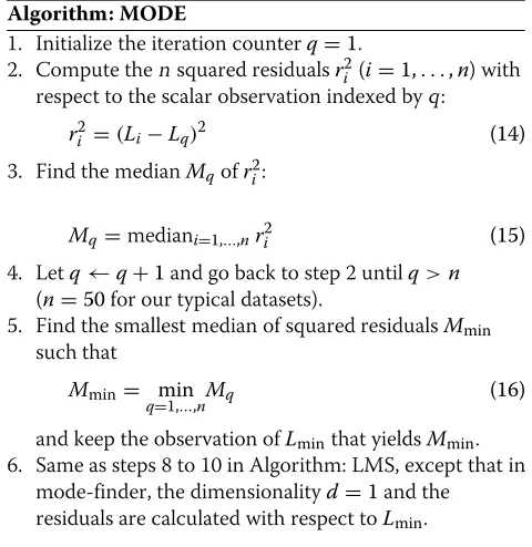
To see how the outlier identification works in the two methods, we study a particular pixel in theBarbdataset (marked by a yellow cross in Figure 2a). In Figure 2b,c, the actual luminance observations at this pixel location from 50 lighting conditions are represented as either black solid dots (if they are identified as inliers) or red crosses (for outliers) and are sorted in ascending order. For comparison, the approximated luminance values are shown as blue circles. An observation is classified as out-lier if (1) its value is outside the inout-lier band, marked with green shade enclosed by blue dashed lines or (2) its approximated value (blue circle) is negative. Note that the major difference between Method:LMS (Figure 2b) and Method:Mode (Figure 2c) is that the 6D polyno-mial model in LMS generates an inlier band that closely approximates the actual data curve, whereas the 1D con-stant model in Method:MODE creates a wider, hori-zontal band. Despite this seemingly crucial difference, Method:MODE as a matter of fact correctly captures most of the outliers identified by Method:LMS. Although Method:MODE may throw away more data points than necessary, it would not negatively affect the accuracy of estimated polynomial coefficients since these unnecessar-ily excluded data points are matte anyway and a robust method is not affected by the sum of squared residuals as in LS.
(a)
10 20 30 40 50
−0.5 0 0.5 1 1.5 2 2.5 3
Luminance
Lights sorted by pixel luminance
(b)
10 20 30 40 50
−0.5 0 0.5 1 1.5 2 2.5 3
Luminance
Lights sorted by pixel luminance
(c)
0.3 0.4 0.5 0.6 0.7 0.25
0.3 0.35 0.4
χ1 χ2
(d)
Figure 2Comparison of outlier detection with LMS and with mode-finding approach.(a)One original image; consider pixel at yellow ‘x’.(b) Outlier detection with 6D to 1D LMS regression. Here, the pixels are displayed in ascending order sorted by luminance. The approximated values are shown as blue circles. Inlier pixel values (at this 1 pixel, over the set of 50 lights) with estimatedˆLvalues that fall within the green inlier band are displayed as black dots and outlier measured luminances, including values with negative luminance estimates that fall below the horizontal line at
L=0, as black dots with red crosses. The blue dashed lines indicate the boundaries of the inlier band automatically identified by LMS.(c)Outlier detection with luminance-mode finder. Here the blue solid line shows the location of the (scalar) mode, bracketed by a horizontal inlier band; inliers also exclude negative-Lˆlights.(d)Red vs. green chromaticity, with outliers for green mode showing red circles (see Section 4.3).
4.3 Luminance versus chromaticity modes
As mentioned earlier in Subsection 4.1, the mode-finder can be applied on luminance but as well could be applied to colour components, since non-matte observations tend to have an altered chromaticity. For example, in Figure 2c, we have shown the outliers iden-tified by Method:MODE on luminance. In Figure 2d, we apply mode-finder on green chromaticity only and find that the observations with outlying green com-ponents (red circles) tend to have outlying red chro-maticities as well. In addition, the chromaticity outliers are also expected to largely overlap with the luminance outliers.
It is also possible to combine outliers obtained from dif-ferent chromaticities or even mix luminance/chromaticity outliers in the hope of getting a more accurate outlier esti-mation. For example, we can estimate outliers using green chromaticity (this subset of outlier indices are denoted cgreen) and red chromaticity (cred) at the same time, and
then take the outlierscthat appear in bothcgreenandcred,
i.e.c=cgreen∩cred. We refer to such a combined method
as ‘green & red’.
Now the question is: which combination of modalities gives the best approximated appearance? We found [46] that in terms of peak signal-to-noise ratio (PSNR) accu-racy of the reconstructed appearance for Method:MODE, we have an ordering:
Lum> (green & red & lum) >green> (green & red) >lum(Method:QUANTILE)
where ‘>’ means better accuracy; using luminance alone is always best, (green & red) seems to be slightly worse than green only, and (green & red & lum) is between green and luminance. In comparison, using luminance with Method:QUANTILE has the worst performance.
5 Higher-dimensional LS-based PTM and hemispherical harmonics
precision recall fMeasure 0.6
0.65 0.7 0.75 0.8 0.85 0.9 0.95 1
Chromaticity Luminance
(a)
0 10 20 30 40
0 0.1 0.2 0.3 0.4 0.5
Deviated angle (degrees)
Occurrence
(b)
0 10 20 30 40 50
0 0.05 0.1 0.15 0.2 0.25 0.3 0.35
Deviated angle (degrees)
Occurrence
(c)
0 0.2 0.4 0.6 0.8 1 0
0.1 0.2 0.3 0.4 0.5 0.6 0.7 0.8
Difference in albedo
Occurrence
(d)
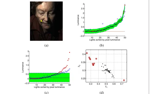
Figure 3Surface properties recovered with mode-finder compared with 6D LMS.(a)Accuracy of outlier detection of mode-finder compared to 6D LMS.(b,c,d)The deviation in surface normal, chromaticity and albedo, respectively.
dimensionality of the classical PTM model above 6D with-out including robust regression. In addition, we apply PTM with different dimensions to model luminance and chromaticity separately. The objective of this part of the investigation is to show that one can, in fact, go quite a long way towards accuracy of appearance modelling using only high-dimensional smooth regression, without the final step of RBF modelling, provided we separate modelling of luminance and chrominance.
Secondly, aside from polynomials, other sets of basis functions can be used to model lighting-surface interac-tion. One notable example is HSH [34] - it has also been suggested that one could replace a PTM polynomial basis by HSH instead [47]. HSH is mathematically very similar to SH which have already been extensively employed in computer graphics. The key difference between HSH and SH is that HSH is only defined for light directions that live on an upper hemisphere, making it more appropriate for our experimental setup.
The conclusions we reach are that (1) a higher dimen-sion does indeed substantially improve the quality of the reconstructed appearance; (2) if we split the problem into modelling luminance and chrominance separately,
rather than applying PTM to each component of colour, then we can reduce the dimensionality for chrominance, compared to that for luminance - we find that 16D for luminance and 9D for chrominance work well; and (3) sur-prisingly, PTM works better than HSH. Note that every dataset we tried behaved this same way.
5.1 Separation of luminance and chromaticity using LS-based PTM
1 4 6 9 16 15
20 25 30 35 40
Number of terms
PSNR
PTM HSH
(a)
1 4 6 9
16
1 4 6 9 16 20 30 40
order (luminance)
order (chromaticity)
HSH PTM
(b)
−1
0 1
−1 0 10 20 40
0 10 20 30 40
(c)
−1
0 1
−1 0 10 20 40
0 10 20 30 40
(d)
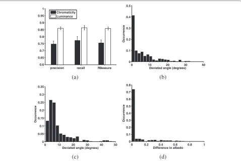
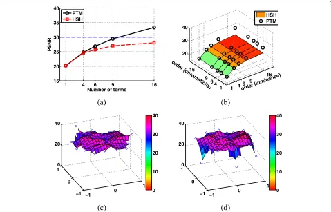
Figure 4Quality of entire image set reconstructed with non-robust, LS-based PTM and HSH over range of dimensionalities.(a)PSNRs for PTM (black curve) and HSH (red, dashed curve), for luminance images, over values of the basis set dimension; the horizontal blue dashed line indicates PSNR = 30. Here the PSNR value displayed is for the entire set of input images compared to the approximated set.(b)PSNRs for PTM (scattered circles) and HSH (surface) in RGB images versus the dimensions for luminance and chromaticity.(c,d)PSNRs for approximated images for each of the lighting direction images, for PTM and HSH, respectively. PSNR is plotted as against thexandycomponents of the lighting direction. Blue circles indicate PSNRs for individual reconstructed image in the dataset, and the coloured surface shows an interpolation surface. Here, 16D for luminance and 9D for chromaticity are used.
acceptable (chosen to be PSNR≥30 dB) reconstruction atd=16.
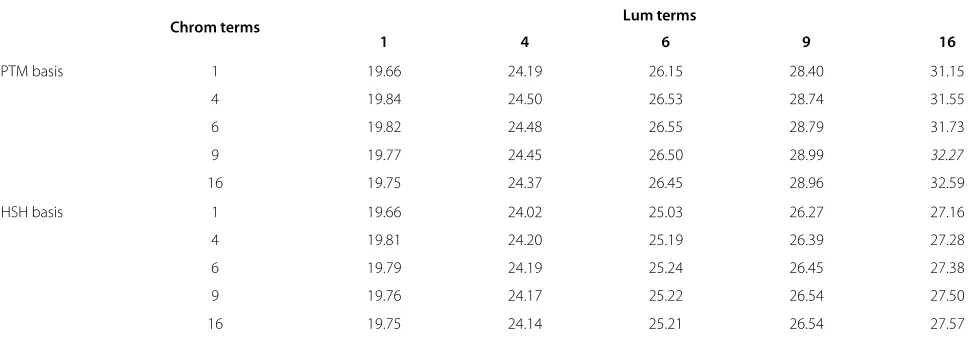
Second, we also investigate modelling the luminance and chromaticity separately, using different dimensionali-ties for each. (Note that only two of the components ofχ need be modelled, since3k=1χk ≡ 1). Figure 4b shows results for dimension of luminance versus chrominance, for HSH (coloured surface) and PTM (black circles). We see that while a higher dimension for luminance is impor-tant (as in Figure 4a), the accuracy of approximation of chrominance is only mildly dependent upon dimension. The actual PSNR values plotted in Figure 4b are shown in Table 1.
Due to the two observations made above, we conclude that the quality of the reconstructed images is mainly determined by the luminance, rather than the chromatic-ities. Hence, in order to achieve a high PSNR with a given dimensionality, it is reasonable to assign a higher sionality for luminance and a relatively lower dimen-sionality for chromaticities. Here we adoptd = 16 for
luminance andd= 9 for chromaticities, making the total number of dimensions 16+9×2=34.
5.2 Comparison of higher-dimension PTM and HSH Using the LS-based approach, we use either a polyno-mial matrixPor an HSH equivalent, which we denote as S. When we solve Equation 3, we also prudently include some Tikhonov regularization [48] in solving for c. The solution of Equation 3 is thus
c = P†L
or c = S†L (17)
where † indicates forming a pseudoinverse using a small amount of regularization, with Tikhonov parameter (denotedτ) of, say,τ =10−3.
We relegate the definition of HSH to Appendix 1. There we list explicitly the definition of the first 16 HSH basis functions, along with the first 16 PTM polynomials.
Table 1 Comparison of PTM and HSH over various dimensionalities
Chrom terms Lum terms
1 4 6 9 16
PTM basis 1 19.66 24.19 26.15 28.40 31.15
4 19.84 24.50 26.53 28.74 31.55
6 19.82 24.48 26.55 28.79 31.73
9 19.77 24.45 26.50 28.99 32.27
16 19.75 24.37 26.45 28.96 32.59
HSH basis 1 19.66 24.02 25.03 26.27 27.16
4 19.81 24.20 25.19 26.39 27.28
6 19.79 24.19 25.24 26.45 27.38
9 19.76 24.17 25.22 26.54 27.50
16 19.75 24.14 25.21 26.54 27.57
PSNR values for least-squares matte regression over ranges of dimensionalities for luminance and chromaticity. The italicized value is obtained with the combination of dimensionalities 16D for luminance and 9D for chromaticity.
dimensiond = 16, HSH still cannot produce an accept-able result. Similar results are shown in Figure 4b and Table 1.
We further compare the PSNR for each individual image in the dataset. Figure 4c,d shows PSNR for approxima-tion of each image in the colour image set, using PTM and HSH, respectively. Here, as described in Section 5.1,d= 16 for luminance andd=9 for chrominance are used. We see that as well as producing higher PSNR values, PTM also does not lose too much accuracy for lighting direc-tions with large incident angles (lights low to the object), whereas HSH does very poorly at these boundary points.
In Table 2 we summarize statistics for PSNRs in Figure 4c,d and as well include results for applying PTM or HSH to each component of RGB separately: to be com-parable with dimensionality of 16 for luminance and 9 for chromaticity (for each of two components), making a total of 34 dimensions, here we model R,G,B with 11D each.
For comparison, we also include results for the RBF modelling in Section 6 below: the PSNR values are not (machine-) infinite because Tikhonov regularization moves the approximation slightly away from exactly reproducing input images.
6 Specularities and shadows: RBF modelling Following [6] we adopt an RBF network approach for the remaining luminance not explained by the matte model Equation 3. For N-pixel images, the ‘excursion’ H is defined as the set of(N×3×n)non-matte colour values not explained by theRmattegiven by the basic PTM matte
Equation 3, now extended to functions of the colour chan-nel as well: the approximated colour matte image is given by
Rmatte = P Cχ, (18)
where C is the collection of all luminance-regression slopes. Since we include colour, all RBF quantities become functions of the colour channel as well. Throughout, we use the mode-finder efficient robust outlier finder to determine coefficientsC.
Then a set of non-matte excursion colour valuesH is defined for our input set of colour images, via H = R − Rmatte where R is the(N × 3× n) set of input
images. We follow [6] in carrying out RBF interpolation for interpolant light directions. But here we use the much
Table 2 Comparison of modelling luminance + chromaticity and RGB
Mean Median Mean bottom quartile Mean top quartile
Lum + Chrom (16D + 9D×2) PTM 32.60 32.80 28.58 36.37
HSH 31.80 32.86 24.67 36.51
RGB (11D×3) PTM 30.35 30.49 25.71 34.20
HSH 30.33 31.28 23.68 34.95
RBF 47.94 46.47 36.60 61.63
faster luminance-mode approach Method:MODE for gen-erating matte images and also for recovering the surface chromaticity, surface normal and albedo.
For a particular input dataset, the RBF network models the interpolated excursion solely based on the direction to a new lighta: an estimate is given byηˆ = RBF(a). Thus, one arrives at an overall interpolant
ˆ
R = ˆRmatte(a) + ˆη(a) (19)
Since in general we do not possess ground-truth data for acquired image sets, we can characterize the accu-racy of appearance-interpolation methods by a leave-one-out analysis. In this approach, we carry leave-one-out the entire image modelling task but omit, in turn, each of the input set images, thus yielding a modelling dimension-ality decreased by 1. Since we know the left-out image’s appearance, we can generate an error characteristic by comparing the interpolated image with the actual one.
We will summarize how to use RBF interpolation and appearance reconstruction in Sections 6.1 and 6.2, respectively. Then in Section 6.3, we present a method to optimize the parameters of the radial Gaussian function, which serves as the third contribution in this work.
6.1 RBF
A brief recapitulation of the RBF calculation is in order, so as to explain the mechanism of developing a leave-one-out error measurement below.
As in [6], we first generate a matte interpolation struc-ture from in-sample input images and then use RBF to model the excursion H, for the part of the input image which cannot be explained by a matte model. So first we model the luminanceL, using either PTM or HSH. E.g. if we decide to use a 16D polynomialp(A), then luminance for in-sample images is modelled byLmatte = C (p(A))†,
whereCis the set of polynomial coefficients. If there are Npixels andnlights, thenLmatteisN×nandCisN×16,
and the polynomial term above is 16×n.
We obtain an N × 3 set of chromaticities as in Equation 12 from which we can generate a matte colour image model for in-sample imagesRmatte, for each if the
i=1..nlighting directions, via
Ri
matte = diag
Li matte
χ, i=1..n (20)
The dimensionality ofRmatteisN ×3×n. The set of
excursions for all the input imagesHhas this same dimen-sionality, andH =R−Rmatte. Because the RBF modelling
adopted in [6] includes a so-called polynomial term (actu-ally, linear here), we have to extendHwith a set ofN×3×4 zeros. Call this extended excursionH.
For interpolation, we need a set of RBF coefficients, with dimensionality N ×3 ×(n+ 4). We adopt Gaus-sian RBF basis functionsφ(a−ai),i = 1..n(although
of course other functions might be tried, such as multi-quadric or inverse-multimulti-quadric). We call the setφ(ai− aj)matrix. Thenis extended into an(n+4)×(n+4) matrixas in [6].
Then we calculate and store the RBF coefficientsover all the input lights as follows:
= H()†
(21)
where the † means the Moore-Penrose pseudoinverse, guarding against reduced rank.
However, here we also extend the pseudoinverse to include some Tikhonov regularization:
()† = T + τI(n +4)
T
(22)
with Tikhonov parameter τ. Below, we mean to opti-mize this parameter using a clever mathematical theorem borrowed for this work.
6.2 Appearance reconstruction
Given a novel lighting directiona, appearance reconstruc-tion from PTM coefficientsCand RBF coefficientsis quite straightforward: we generate a matte image by mul-tiplying PTM coefficient matrix C by its corresponding combination of polynomialp(a)and then use recovered chromaticityχ to form a colour matte image. Then we form a new Gaussian functionφfrom new lighting direc-tion a and simply multiply φ times the prestored RBF excursion coefficient set to generate a single-image excursion valueη. The Gaussian radial basis function has the explicit formφ(ai,aj,σ)=exp(−r2/σ2), with radiusr for light-direction vectorsaiandajgiven byr= ai−aj.
6.3 Optimization of dispersionσand of Tikhonov parameterτ
In this subsection, we describe our third contribution, i.e. finding the best values for the Gaussian dispersionσand the Tikhonov coefficient τ so as to optimize the recon-structed appearance. Since we have no ground truth for real input image sets, we test the accuracy of appearance modelling by simply leaving out one of theninput images at a time and attempting to reconstruct the left-out image. To this end, here we borrow the work in [49] in deter-mining a best value of the Gaussian dispersion parameter σ to minimize the leave-one-out error. However, here we mean to apply the method given in [49] to a whole image at once and include colour, extend RBF modelling to include the additional polynomial term and, finally and impor-tantly, extend [49] to include Tihkonov regularization and its optimization.
E.g. if the input set consists of 50 images, then we fol-low through matte and then RBF modelling using only 49 images and attempt to reconstruct the 50th image, and then repeat for each of the 50 light directions.
Modelling on the theorem given in [49] in Appendix 2, we generalize the theorem, which is aimed at optimiz-ing RBF over the dispersion parameterσ, to also optimize over Tikhonov parameter τ. The resulting calculation from this theorem is so fast that it is simple to run any unconstrained non-linear optimizer such as the subspace trust-region method [50].
We find that an approximate colour image reconstruc-tion, for thekth leave-one-out image, is simply as follows:
E = /v
ˆ
R = R − E
(23)
where theerror imageEis simply formed from the RBF coefficients, and a vectorvgenerated as the solution to the following simple equation in terms of the(n+4)× (n+4)identity matrixI:
v = I (24)
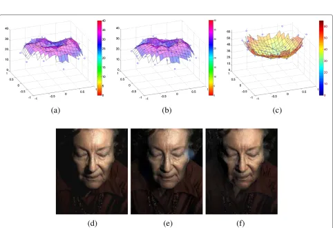
This theorem means that one can very rapidly assess the error generated in a leave-one-out analysis of RBF mod-elling. Figure 5a shows the PSNR between the actual input image set and the result of matte plus RBF modelling, for an optimal choice ofσ andτ. Unsurprisingly, we see that RBF interpolation does best in the center of the cluster of lighting directions and worse when there is less sup-porting information, near the boundary of the cluster of light directions. We take as the optimum dispersionσand Tihkonov parameter value τ as those which deliver the highest leave-one-out median PSNR over the set overall.
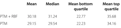
Table 3 shows PSNR statistics for this leave-out-out RBF test. In comparison, we show in Figure 5b and also in the second line of Table 3 the results of a leave-one-out test using PTM matte modelling alone for dimensions 16 and 9 for luminance and chrominance, with no RBF stage. We notice that in a challenging leave-one-out test for inter-polation, PTM does reasonably well. To put these plots in perspective, in Figure 5c, we also show the results for PTM + RBF in a leave-all-in setting: of course, the PSNR for PTM + RBF for leave-all-in is by far the best accuracy. In Figure 5d we show the in-sample correct image closest to the mean value of PSNR values for all leave-one-out RBF
Table 3 PSNR statistics for leave-one-out test, using PTM + RBF, and using only PTM
Mean Median Mean bottom Mean top quartile quartile
PTM + RBF 30.18 31.24 22.77 35.68
PTM 29.15 29.54 22.23 34.16
modelling, and in Figure 5e,f, we show the interpolants from using PTM + RBF and from using just PTM, respec-tively. Clearly, RBF provides a substantial boost in visual appearance, although PTM itself (with no RBF stage), with the higher dimensions we have specified, does produce a reasonable image. Nevertheless, qualitatively, using RBF does much better in that, without RBF, specularities are not well modelled and the shadows are wrong.
7 Conclusions
In this paper, we have set out tests and conclusions that improve PTM modelling for appearance interpolation and surface property recovery. We found that increasing PTM dimensionality has a substantial effect on accuracy, more for the luminance channel than for colour. We found that a dimension of 16 for luminance and 9 for chromaticity, modelling luminance and chromaticity separately, deliv-ered good performance. We found that for determining outliers, we could have almost as good accuracy using a much less burdensome robust 1D ‘location finder’ as in a more accurate but slower robust multivariate processing.
A second stage of modelling using RBF interpolation provides a large boost in accuracy of appearance mod-elling. Here we showed that Tikhonov regularization in calculating RBF coefficients was important, since we are inverting large matrices; and moreover we incorporated optimizing the Tikhonov parameter into an optimization theorem that had been initially aimed at only generating a best choice of Gaussian dispersion parameter for radial basis function networks.
Future work will include developing a real-time viewer including the new insights gained here.
Appendix 1: hemispherical harmonics
HSH are derived from spherical harmonics (SH) as an alternative set of basis functions on the unit sphere that are particularly aimed at non-negative function values. The familiar SH are defined as [51]
Ylm(θ,φ)=KlmeimφPl|m|cos(θ),l∈N,−l≤m≤l (25)
where θ ∈[ 0,π] is the altitude angle, and φ ∈[ 0, 2π] the azimuth angle. Plm are the associated Legendre
polynomials, orthogonal polynomial basis functions over [−1,+1], andKlmare the normalization factors for these.
Pml (x)= (−21ll)!m
(1−x2)m d(l+m)
dx(l+m)(x2−1)l
Klm=
(2l+1)(l−|m|)! 4π(l+|m|)!
(26)
In the context of computer graphics, real-valued functions as follows are often preferred:
Ylm=
⎧ ⎨ ⎩
√
2Klmcos(mφ)Pml (cosθ), m>0 √
2Klmsin(−mφ)P−l m(cosθ), m<0 Kl0P0l(cosθ), m=0
(27)
However, since in graphics the incident and reflected lights are all distributed on an upper hemisphere, it requires a large number of coefficients to handle the dis-continuities at the boundary of the hemisphere when the mapping is represented with basis defined on a full sphere [34]. Thus, it is more natural to use an HSH basis instead. In this study, we used the HSH model proposed in [34]n:
Hlm=
⎧ ⎨ ⎩
√
2K˜lmcos(mφ)P˜ml (cosθ) m>0 √
2K˜lmsin(−mφ)P˜l−m(cosθ) m<0 ˜
Kl0P˜l0(cosθ) m=0
(28)
where P˜ml and K˜lm are the ‘shifted’ associated Legendre polynomials and the hemispherical normalization factors, respectively, defined as follows:
˜
Pml (x)=Pml (2x−1)
Klm=
(2l+1)(l−|m|)! 2π(l+|m|)!
(29)
Now the hemispherical functions are defined only over the upper hemisphere,θ ∈[ 0,π/2] ,φ∈[ 0, 2π].
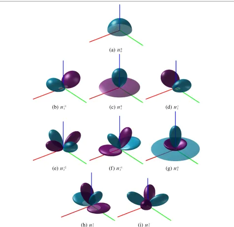
Figure 6 shows the first three ‘bands’ of the HSH, i.e. l = 0..2, and the first 16 functions are stated explicitly in Equation 31.
Similarly, we can also consider the polynomial basis in Equation 1 as a set of functions defined on the hemi-sphere by representing the lighting direction (u,v,w) with spherical polar coordinates:u = sinθcosφ,v = sinθsinφ,w= cosθ, so e.g. the PTM basis functions in Equation 1 are given by
(sinθcosφ, sinθsinφ, cosθ, sin2θcos2φ, sin2θcosφsinφ, 1) (30)
Hi=Hlm;i=((l+1)l−m)+1; Order=(l+1): Order 1:
H1(θ,φ)=1/√(2π)
Order 2: H2(θ,φ)=
√
(6/π)(cos(φ)√(cos(θ)−cos(θ)2))
H3(θ,φ)=√(3/(2π))(−1+2 cos(θ))
H4(θ,φ)=√(6/π)(sin(φ)√(cos(θ)−cos(θ)2))
Order 3:
H5(θ,φ)=√(30/π)(cos(2φ)(−cos(θ)+cos(θ)2))
H6(θ,φ)= √
(30/π)(cos(φ)(−1+2 cos(θ)) √
(cos(θ)−cos(θ)2))
H7(θ,φ)=√(5/(2π))(1−6 cos(θ)+6 cos(θ)2)
H8(θ,φ)= √
(30/π)(sin(φ)(−1+2 cos(θ)) √
(cos(θ)−cos(θ)2))
H9(θ,φ)=√(30/π)((−cos(θ)+cos(θ)2)sin(2φ))
(31)
Order 4:
H10(θ,φ)=2√(35/π)cos(3φ)(cos(θ)−cos(θ)2)3/2
H11(θ,φ)= √
(210/π)cos(2φ)
(−1+2 cos(θ))(−cos(θ)+cos(θ)2) H12(θ,φ)=2√(21/π)cos(φ)√(cos(θ)−cos(θ)2)
(1−5 cos(θ)+5 cos(θ)2) H13(θ,φ)=√(7/(2π))(−1+12 cos(θ)−30
cos(θ)2+20 cos(θ)3)
H14(θ,φ)=2√(21/π)sin(φ)√(cos(θ)−cos(θ)2)
(1−5 cos(θ)+5 cos(θ)2)
H15(θ,φ)= √
(210/π)(−1+2 cos(θ))(−cos(θ)+ cos(θ)2)sin(2φ)
H16(θ,φ)=2√(35/π)sin(3φ)(cos(θ)−cos(θ)2)3/2
Constant term: P1 = 1
Linear terms:
P2 = u = sin(θ)cos(φ)
P3 = v = sin(θ)sin(φ)
P4 = w = cos(φ)
Quadratic terms:
P5 = u2 = sin2(θ)cos2(φ)
P6 = uw = sin(θ)cos2(φ)
P7 = uv = sin2(θ)cos(φ)sin(φ)
P8 = vw = sin(θ)cos(φ)sin(φ)
P9 = v2 = cos2(φ)
(32)
Cubic terms:
P10 = u3 = sin3(θ)cos3(φ)
P11 = u2v = sin3(θ)cos2(φ)sin(φ)
P12 = u2w = sin2(θ)cos3(φ)
P13 = uvw = sin2(θ)cos2(φ)sin(φ)
P14 = v2u = sin3(θ)sin2(φ)cos(φ)
P15 = v2w = sin2(θ)sin2(φ)cos(φ)
P16 = v3 = sin3(θ)sin3(φ)
Appendix 2: leave-one-out optimization in RBF It is useful to state explicitly how the optimization theorem in [49] goes over to the situation when Tikhonov regularization comes into play.
Firstly, we utilize three-band colour image data, rather than scalar data, and process whole images at once using vectorized programming in Matlab. However for clarity, below we state matters as they pertain to a single pixel and in one colour band.
Suppose there arenlights andninput values at a pixel, e.g. for our exemplar dataset n = 50. Then we make (n+4)×(n+4)matrix(σ), where here we are explic-itly including dependence on a variable dispersion valueσ. For the(n+4)vector of excursion valuesH(extended by four zeros to include the ‘polynomial’ RBF part), we begin by solving for the(n+4)vector set of RBF coefficientsψ, which is the vector solution for the modelling equation
H = ψ
However, instead of simply using a matrix inverse in order to guard against numerical instability, we make use of the Tikhonov regularized inverse from Equation 22:
ψ = (σ,τ)†H
so that in fact we generate only approximate, not exact, approximationsHˆ for in-sample lighting directions:
ˆ
H = ψ = †H
Then the main task is interpolation to any new lightavia
η = (n+4)
j=1
ψT
j φ(aj−a)
whereηis the scalar value of interpolated excursion (for this pixel and colour channel).
Now we mean to consider the leave-one-out problem, meaning that all the matrices and vectors have extent (n + 3)because thekth input-image case has been omit-ted. Suppose we denote this case using superscript (k). That is, we aim for a solutionψ(k)of
H(k) = (k)ψ(k) (33)
Firstly, consider the following Lemma: if vectorv has vk=0, then
(a)
H0 0(b)
H-11
(c)
H10(d)
H11(e)
H-22
(f)
H2-1(g)
H20(h)
H12
(i)
H22Figure 6Visualization of the first three bands of hemispherical harmonics.(a)H00.(b)H−11.(c)H01.(d)H11.(e)H2−2.(f)H−21.(g)H20.(h)H12.(i)H22. The distancerfrom the origin to any point(θ,φ,r)on the plot surface is proportional to the value ofHm
l at direction(θ,φ), with cyan indicating
positive values and purple negative. Red, green and blue indicatex,yandzaxes, respectively.
That is, if we know the not-reduced-dimension equation holds, then for the special situation in whichvk = 0, we can simply omit whatever valuebk may take on, for the reduced-dimension problem indicated by(k).
Now consider an auxiliary full-dimension vector v defined such that
v=+ek
whereekis thekth column of the unit matrix.
Now define a new vector
β = ψ − (ψk/vk)v
Notice that thekth component ofβis zero. Now evaluateβ:
(a)1
(b) (c) (d)
(e) (f) 2 (g)
(h) 2 (i) 3
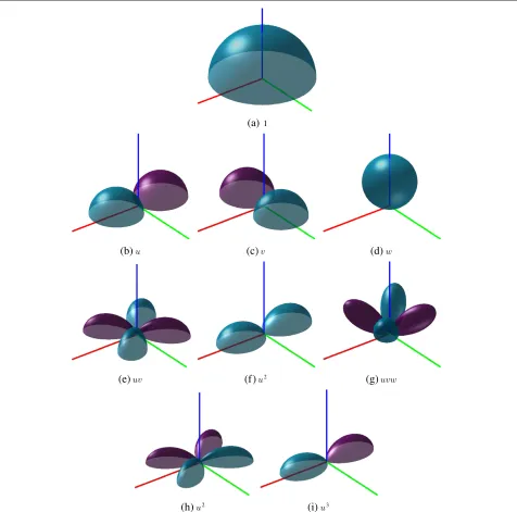
Figure 7Visualization of selected polynomial basis functions.(a)1,(b)u,(c)v,(d)w,(e)uv,(f)u2,(g)uvw,(h)u2,(i)u3. The distancerfrom the origin to any point(θ,φ,r)on the plot surface is proportional to the value of the polynomial termPat direction(θ,φ), with cyan indicating positive values and purple negative. Red, green, blue indicatex,y,zaxes, respectively.
Hence, by our lemma, β is the sought solution for the leave-one-out set of coefficientsψ(k); however, this state-ment is approximate and not exact because ηˆ is only approximately (but very close to being equal to)η.
So in order to optimize onσ and τ, we need only to generate the error estimateEkfor thekth case,
Ek = −(ψk/vk)
for each of thek = 1..nleft-out lights, and apply some appropriate error measure such as median (Ek) for choos-ing the least-error solution:
min {σ,τ}
n median
k=1 Ek(σ,τ) (34)
general interpolation for the dataset being optimized for by this leave-one-out procedure.
Competing interests
The authors declare that they have no competing interests.
Received: 10 August 2013 Accepted: 16 April 2014 Published: 1 May 2014
References
1. T Malzbender, D Gelb, H Wolters, Polynomial texture maps, inProceedings of Computer Graphics, SIGGRAPH, vol. 2001 (ACM Los Angeles, California, 2001), pp. 519–528
2. RJ Woodham, Photometric method for determining surface orientation from multiple images. Opt. Eng.19, 139–144 (1980)
3. M Mudge, T Malzbender, C Schroer, M Lum, New reflection transformation imaging methods for rock art and multiple-viewpoint display, in7th International Symposium on Virtual Reality, Archaelogy and Cultural Heritage(Eurographics, Nicosia, Cyprus, 2006)
4. K Sunkavalli, T Zickler, H Pfister, Visibility subspaces: uncalibrated photometric stereo with shadows, in11th European Conference on Computer Vision–ECCV 2010(Springer Heraklion, 2010), pp. 251–264 5. G Earl, K Martinez, T Malzbender, Archaeological applications of
polynomial texture mapping: analysis, conservation and representation. J. Archaeological Sci.37, 1–11 (2010)
6. M Drew, Y Hel-Or, T Malzbender, N Hajari, Robust estimation of surface properties and interpolation of shadow/specularity components. Image Vis. Comput.30(4-5), 317–331 (2012)
7. PJ Rousseeuw, AM Leroy,Robust Regression and Outlier Detection. (Wiley, New York, 1987)
8. T Zickler, S Enrique, R Ramamoorthi, P Belhumeur, Reflectance sharing: image-based rendering from a sparse set of images, inEurographics Symposium on Rendering Techniques(Konstanz, Germany, 2005), pp. 253–265
9. T Zickler, R Ramamoorthi, S Enrique, P Belhumeur, Reflectance sharing: predicting appearance from a sparse set of images of a known shape. IEEE Trans. Patt. Anal. Mach. Intell.28, 1287–1302 (2006)
10. EN Coleman Jr, R Jain, Obtaining 3-dimensional shape of textured and specular surfaces using four-source photometry. Comput. Graph. Image Process.18, 309–328 (1982)
11. F Solomon, K Ikeuchi, Extracting the shape and roughness of specular lobe objects using four light photometric stereo. IEEE Trans. Patt. Anal. Mach. Intell.18, 449–454 (1996)
12. S Barsky, M Petrou, The 4-source photometric stereo technique for three-dimensional surfaces in the presence of highlights and shadows. IEEE Trans. Patt. Anal. Mach. Intell.25(10), 1239–1252 (2003)
13. H Rushmeier, G Taubin, A Guéziec, Applying shape from lighting variation to bump map capture, inEurographics Rendering Techniques 97(Springer Vienna, 1997), pp. 35–44
14. A Yuille, D Snow, Shape and albedo from multiple images using integrability, inProceedings of the IEEE Computer Society Conference on Computer Vision and Pattern Recognition 1997(San Juan, Puerto Rico, 1997), pp. 158–164
15. G Willems, F Verbiest, W Moreau, H Hameeuw, K Van Lerberghe, L Van Gool, Easy and cost-effective cuneiform digitizing, inProceedings of 6th International Symposium on Virtual Reality, Archaeology and Cultural Heritage (Short and Project Papers)(Pisa, Italy, 2005), pp. 73–80
16. J Sun, M Smith, L Smith, S Midha, J Bamber, Object surface recovery using a multi-light photometric stereo technique for non-Lambertian surfaces subject to shadows and specularities. Image Vis. Comput.25, 1050–1057 (2007)
17. Julià C, F Lumbreras, AD Sappa, A factorization-based approach to photometric stereo. Int. J. Imag. Syst. Tech.21, 115–119 (2011) 18. L Wu, A Ganesh, B Shi, Y Matsushita, Y Wang, Y Ma, Robust photometric
stereo via low-rank matrix completion and recovery, inComputer Vision – ACCV 2010, ed. by Kimmel R, Klette R, Sugimoto A, and Lecture notes in computer science, no. 6494. (Springer Berlin Heidelberg, 2011), pp. 703–717
19. KL Tang, CK Tang, TT Wong, Dense photometric stereo using tensorial belief propagation, inIEEE Computer Society Conference on Computer
Vision and Pattern Recognition 2005, vol. 1 (San Diego, California, 2005), pp. 132–139
20. M Chandraker, S Agarwal, D Kriegman, ShadowCuts: photometric stereo with shadows, inIEEE Computer Society Conference on Computer Vision and Pattern Recognition 2007(Minneapolis, Minnesota, 2007), pp. 1–8 21. F Verbiest, L Van Gool, Photometric stereo with coherent outlier handling
and confidence estimation, inIEEE Computer Society Conference on Computer Vision and Pattern Recognition 2008(Anchorage, Alaska, 2008), pp. 1–8
22. Q Yang, N Ahuja, Surface reflectance and normal estimation from photometric stereo. Comput. Vis. Image Underst.116(7), 793–802 (2012) 23. S Kherada, P Pandey, A Namboodiri, Improving realism of 3D texture
using component based modeling, in2012 IEEE Workshop on Applications of Computer Vision (WACV)(Breckenridge, Colorado, 2012), pp. 41–47 24. SH Westin, JR Arvo, KE Torrance, Predicting reflectance functions from
complex surfaces, inProceedings of the 19th Annual Conference on Computer Graphics and Interactive Techniques,SIGGRAPH ‘92 (New York, 1992), pp. 255–264
25. TT Wong, PA Heng, SH Or, WY Ng, Image-based rendering with controllable illumination, inProceedings of the Eurographics Workshop on Rendering Techniques 1997(Springer Vienna, 1997), pp. 13–22 26. JS Nimeroff, E Simoncelli, J Dorsey, Efficient re-rendering of naturally
illuminated environments, inPhotorealistic Rendering Techniques, Focus on Computer Graphics(Springer Berlin Heidelberg, 1995), pp. 373–388 27. J Kautz, PP Sloan, J Snyder, Fast, arbitrary BRDF shading for low-frequency
lighting using spherical harmonics, inProceedings of the 13th Eurographics Workshop on Rendering Techniques(Pisa, Italy, 2002), pp. 291–296 28. R Ramamoorthi, P Hanrahan, An efficient representation for irradiance
environment maps, inProceedings of the 28th Annual Conference on Computer Graphics and Interactive Techniques(Los Angeles, California, 2001), pp. 497–500
29. PP Sloan, J Kautz, J Snyder, Precomputed radiance transfer for real-time rendering in dynamic, low-frequency lighting environments, inACM Transactions on Graphics (TOG), vol. 21 (ACM, New York, 2002), pp. 527–536 30. PP Sloan, J Sloan, J Hart, J Snyder, Clustered principal components for
precomputed radiance transfer. ACM Trans. Graph.22(3), 382–391 (2003) 31. R Basri, DW Jacobs, Lambertian reflectance and linear subspaces. IEEE
Trans. Patt. Anal. Mach. Intell.25, 218–233 (2003)
32. R Basri, D Jacobs, I Kemelmacher, Photometric stereo with general, unknown lighting. Int. J. Comput. Vis.72, 239–257 (2007) 33. L Zhang, D Samaras, Pose invariant face recognition under arbitrary
unknown lighting using spherical harmonics, inBiometric Authentication. Lecture notes in computer science, vol 3087(Springer Heidelberg, 2004), pp. 10–23
34. P Gautron, J Kˇrivánek, SN Pattanaik, K Bouatouch, A novel hemispherical basis for accurate and efficient rendering, inEurographics Symposium on Rendering Techniques 2004(Eurographics Association, Norköping, Sweden, 2004), pp. 321–330
35. S Elhabian, H Rara, A Farag, 2011 Canadian Conference on Computer and Robot Vision (CRV) (St. Johns, Newfoundland, 2011), pp. 293–300 36. H Huang, L Zhang, D Samaras, L Shen, R Zhang, F Makedon, J Pearlman,
Hemispherical harmonic surface description and applications to medical image analysis, inThird International Symposium on 3D Data Processing, Visualization, and Transmission(Chapel Hill, North Carolina, 2006), pp. 381–388
37. S Elhabian, H Rara, A Farag, Towards accurate and efficient representation of image irradiance of convex-Lambertian objects under unknown near lighting, in2011 IEEE International Conference on Computer Vision (ICCV)
(Barcelona, Spain, 2011), pp. 1732–1737
38. G Earl, K Martinez, T Malzbender, Archaeological applications of polynomial texture mapping: analysis, conservation and representation. J. Archaeol. Sci.37(8), 2040–2050 (2010)
39. G Earl, G Beale, K Martinez, H Pagi, Polynomial texture mapping and related imaging technologies for the recording, analysis and presentation of archaeological materials, inISPRS Commission V Midterm Symposium
(Newcastle, 21–24 June 2010), pp. 218–223
40. G Earl, PJ Basford, AS Bischoff, A Bowman, C Crowther, J Dahl, M Hodgson, K Martinez, L Isaksen, H Pagi, KE Piquette, E Kotoula, Reflectance transformation imaging systems for ancient documentary artefacts, in