https://doi.org/10.5194/jsss-7-245-2018
© Author(s) 2018. This work is distributed under the Creative Commons Attribution 4.0 License.
Calibration of tri-axial MEMS accelerometers in the
low-frequency range – Part 1: comparison
among methods
Giulio D’Emilia1, Antonella Gaspari1, Fabrizio Mazzoleni2, Emanuela Natale1, and Alessandro Schiavi2 1Department of Industrial and Information Engineering and of Economics, University of L’Aquila,
L’Aquila, 67100, Italy
2INRiM - National Institute of Metrological Research, Turin, 10135, Italy
Correspondence:Giulio D’Emilia ([email protected])
Received: 8 February 2018 – Revised: 26 March 2018 – Accepted: 28 March 2018 – Published: 6 April 2018
Abstract. Two alternative experimental procedures for the calibration of tri-axial accelerometers have been compared with traditional methods, performed according the procedures stated in the standard ISO 16063-21. Standard calibration is carried out by comparison with a laser Doppler vibrometer (LDV), used as a primary reference transducer. The main sensitivities have been investigated and, where applicable, also transverse ones. Many aspects have been evaluated: the hypotheses about transverse sensitivities, the simplicity of the procedure, the number of measurements needed, and the effect of typology of transducer, depending on electrical and geometrical contributions. Two different accelerometers have been tested, a piezo-electric accelerometer and a capacitive MEMS accelerometer. A low-frequency range of vibration has been investigated, 3 and 6 Hz, with amplitude of acceleration ranging from 2 to 20 ms−2. A satisfactory reproducibility of methods has been verified, with percentage differences less than 2.5 %. Anyway, pros and cons of each method are also discussed with reference to their possible use for easy and quick calibration of low-cost tri-axial accelerometers.
1 Introduction
In recent years, there has been a growing interest in micro-electro-mechanical system accelerometers (MEMS), due to their low cost, the possibility of embedding these devices within wireless sensor networks, and the capability of detect-ing low-amplitude and low-frequency vibrations, operations which are not always feasible with the conventional low-cost sensor boards (Batista et al., 2011; Sabato et al., 2017). It should be considered that MEMS accelerometers, in com-parison to high-performance piezo-electric transducers, ex-hibit lower accuracy in consumer grade applications; how-ever, in the context of extensive applications, such as large sensor networks, in which high accuracy on a wide range of frequency and amplitude is not needed, the technical per-formances of these accelerometers are considered adequate (Schiavi et al., 2015).
Low-frequency vibration measurements are of great in-terest in many different fields such as, for instance, energy
production (Ripper et al., 2017), structural health monitor-ing (SHM) of buildmonitor-ings and of civil infrastructures (Sabato et al., 2017; Ranieri et al., 2013), and geotechnical applica-tions (Czech and Gosk, 2017) in the field of human vibra-tion and bio-dynamics (Griffin, 2014), mainly because of the increasing development of MEMS embedded in mobile de-vices (Halim and Park, 2013) and in applications in the field of the Internet of Things (IoT) (Borgia, 2014).
The evaluation of sensitivities is a key point of the vi-bration measurements for MEMS accelerometers, and it quires adequate attention from the design phase up to the re-alization and the use of this kind of sensor.
pos-sibility of developing procedures that could be implemented both on-line and in-line (Frosio et al., 2009, 2012; Glueck et al., 2012; Fong et al., 2008).
On-line calibration refers to the possibility of calibrating during assembly in industrial processes, for continuous mon-itoring and controlling of processes. In-line calibration refers to the calibration of sensors installed on an industrial plant, directly carried out on the production line to be monitored without moving it to a laboratory.
The possibility of calibrating sensors in the field is an in-teresting issue not only for practical and economic reasons, but also from a technical point of view. In fact, the MEMS sensor output depends on temperature and, in general, on other environmental conditions (Wu et al., 2002). Therefore, these accelerometers have to be calibrated in the field when a realistic assessment of the measurement uncertainty is an important requirement (Frosio et al., 2009, 2012; Glueck et al., 2012; Fong et al., 2008).
The research for new methods for the on-line and in-line calibration of MEMS is confirmed as one of the points of main relevance. In fact, some procedures are proposed based on different algorithms. In Chen and Han (2011) the wavelet neural network is used for optimizing and compen-sating for the variation of the MEMS acceleration sensors due to temperature change. Rohac et al. (2015) propose a method for calibration of MEMS tri-axial inertial sensors, using a gravity-based calibration method under static condi-tions. Geist et al. (2017) propose a methodology based on the linearization, used for the reduction of the measurement error of the device. The optimization algorithm is validated on an experimental set-up, considering the accelerometer in static state, and rotating it randomly in 30 different orien-tations. These methods are static-based methods and do not consider aspects arising from the experimental practice (e.g. the dynamic behaviour of the phenomena analysed).
In summary, the following main requirements for testing and calibration of accelerometers for the above-mentioned applications should be met:
– to lower the cost of calibration and testing (low-cost cal-ibration);
– to enhance the sensors’ operability, also in dynamic conditions, similar to those of their actual use (dynamic conditions);
– to guarantee the traceability of the methodology, up to the primary calibration (traceability);
– to streamline the production process and to reduce loss in times and costs of possible deviations from the vali-dated information, also in the case of on-line and in-line calibration (on-line and in-line calibration);
– to avoid complex models and algorithms, in order to be easily transferred onto the field, thus increasing their op-erability (simplicity and opop-erability).
A quantitative comparison among three methods is carried out. Two methods have been selected that are potentially able to fulfil the above-mentioned requirements, in a differ-ent way, with respect to the standard method, used as a refer-ence. The standard method, Method 1, is performed accord-ing to the procedures stated in the ISO Standard 16063 se-ries (ISO 1, 1998; ISO 11, 1999; ISO 16063-21, 2003; ISO 16063-31, 2009), to support the traceability. The second one, Method 2 (Schiavi et al., 2015), allows us to determine the three main sensitivities, simultaneously. The last one (Method 3; D’Emilia et al. ,2015, 2016a, b) gives the possibility of obtaining the main sensitivities, transverse sensitivities and offset terms.
In Sect. 2, the methods are described and a discussion of the way each method fits the above requirements is car-ried out. In Sect. 3, the test bench used for the experimental set-up, together with the typology of the accelerometers that have been used, and the planned tests are outlined. The indi-cators used for the comparison purposes are also identified. In Sect. 4 the results for the two typologies of sensors anal-ysed are presented and discussed. Conclusions and hints for future works end the paper.
2 Calibration methods
In the following sections, the methods of calibration and the parameters considered for the comparison will be shown. Then, the test bench used for the experimental tests will also be described.
2.1 Method 1: the standard ISO 16063 series
The standard (ISO 16063-1, 1998) defines the sensitivity for a linear transducer as the ratio of the input during sinusoidal excitation, parallel to a specified axis of sensitivity at the mounting surface.
The procedure to be used for primary calibration of rec-tilinear accelerometers to obtain magnitude and phase lag of the complex sensitivity by steady-state sinusoidal vibra-tion and laser interferometry is described in ISO 16063-11 (1999). The sinusoidal motion applied by the vibration generator is along a well-defined straight line, with negligi-ble lateral motions.
In this paper, the traceability to primary national standards through a secondary standard is accomplished by applying the specifications in ISO 16063-21 (2003). Additionally, the standard (ISO 16063-31, 2009) defines the transverse sensi-tivity of an accelerometer,ST, as the sensitivity to
acceler-ation applied at right angles to its geometric axis. ST,
cor-responding to a specific test direction, is calculated as (1), whereVˆoutis the amplitude of the output signal of the
trans-ducer andaˆTis the amplitude of the acceleration in the test
sensitivity.
ST=
ˆ
Vout
ˆ
aT
(1)
The standard ISO 16063-31 (2009) deals with uni-axial ac-celerometers, excited along directions perpendicular to their sensitive axes.
Extending the indications of the standard to the case of a tri-axial accelerometer, each axis of the sensor could be tested by applying a known acceleration to another axis, with the purpose of calculating according to Eq. (1) the transverse sensitivity of the first axis when excited along the direction of the second one.
Then, by exciting each single axis of a sensor, it is possi-ble to calculate six transverse sensitivities, which express the effect of the acceleration along a single axis, with respect to the other ones.
These transverse sensitivities will be indicated asSxy,Sxz,
Syx,Syz,Szx, andSzy, where the first subscript indicates the axis with reference to which the sensitivity is calculated, and the second one indicates the direction of the excitation.
A similar approach is applied for the determination of the magnitude of the acceleration sensitivities (Sxx, Syy, Szz). The phase lag is assumed to be negligible.
As an example, when the vibration is according to the
xaxis, the sensitivity is calculated as Eq. (2), while the trans-verse sensitivities Syx andSzx can be evaluated as Eqs. (3) and (4), whereVx,Vy andVzare the amplitudes of thex,y andzoutputs of the accelerometer under test, and ax is the amplitude of the reference signal in thexdirection.
Sxx=
Vx
ax
(2)
Syx=
Vy
ax
(3)
Szx=
Vz
ax
(4)
The same procedure is used for the other sensitivities, when the vibration is along the y axis (Syy,Sxy,Szy) andzaxis (Szz,Sxz,Syz), respectively.
2.2 Method 2
Method 2 involves the simultaneous excitation of the three axes of the accelerometer under test.
For this purpose, the accelerometer has to be mounted onto the surface of a clamp, inclined at an angleθ=35◦with re-spect to the horizontal plane (Fig. 1) on which the motion is realized; furthermore, the accelerometer has to be rotated on the clamp surface with an angleα=45◦, in order to si-multaneously excite the three axes in the same way, with a single horizontal sinusoidal acceleration (Fig. 1) (Schiavi et al., 2015).
Figure 1.Inclined clamp – scheme.
In this way, accelerations of similar amplitude are realized along the three axes, which can be simultaneously calibrated. The reference accelerations along the three axes can be obtained as follows in Eqs. (5), (6) and (7):
ax= −aref·cos (θ)·sin(α), (5)
ay= −aref·cos (θ)·cos(α), (6)
az=aref·sin(θ), (7)
wherearefis the acceleration in the motion direction,
mea-sured by a reference sensor.
The output signal and the reference one are analysed by the fast Fourier transform in correspondence to the oscilla-tion frequency, with the purpose of evaluating their spectral amplitudes. The constant terms, gravity-dependent, do not affect the results.
Sxxis evaluated according to Eq. (2), whereVxis the spec-tral amplitude of the output signal of thex axis of the ac-celerometer under test, andax is the spectral amplitude of the reference signal in the same direction.
The same approach allows us to evaluateSyyandSzz, re-spectively, when the other measuring axes of the accelerom-eter are considered.
This approach does not allow us to calculate the transverse sensitivities, since similar acceleration components are re-alized along all axes, simultaneously, without the possibil-ity of extracting the effect of transverse sensitivities. A peri-odic verification that the transverse sensitivities are negligi-ble (< 5 % with respect to the main sensitivities) is necessary for the typology of sensor considered, according to Method 1, described in Sect. 2.1.
2.3 Method 3
This method is based on the following model, describing the relation between the input accelerations and the output sig-nals (Eq. 8), whereV=(Vi) is the output array,A=(ai) is the reference accelerations array,S=(Sij) is the sensitivity matrix andQ=(qi) represents the offset array.
Vx Vy Vz =
Sxx Sxy Sxz
Syx Syy Syz
Szx Szy Szz · ax ay az + qx qy qz (8)
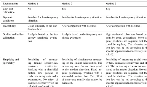
Table 1.Pros and cons of the methods with respect to requirements.
Requirements Method 1 Method 2 Method 3
Low-cost calibration
No Yes Yes
Dynamic conditions
Suitable for low-frequency vibration
Suitable for low-frequency vibration Suitable for low-frequency vibration
Traceability Close similarity to the stan-dard method
After comparison with Method 1 After comparison with Method 1
On-line and in-line calibration
Analysis based on the fre-quency amplitude evalua-tion
Analysis based on the frequency am-plitude evaluation
High statistical robustness based on a point-by-point comparison. More an-gular positions are required, but they could be anything. The vibration mo-tion law can be set according to the specific application (not necessary sinu-soidal).
Simplicity and operability
Possibility of measur-ing (main) sensitivities, transverse sensitivities. Working with a sinusoidal motion law parallel to each measuring axis under examination. No effect of transverse sensitivity on the calculation of sensitivity.
Possibility of simultaneous measur-ing of the (main) sensitivities. The measuring axes do not correspond to the motion direction. Fixed an-gular positioning. Working with a sinusoidal motion law. The effect of transverse sensitivities cannot be evaluated.
Possibility of measuring (main) sensi-tivities, transverse sensitivities and off-set. The measuring axes do not corre-spond to the motion direction. More an-gular positions are required, but they could be whatever. The vibration mo-tion law can be set according to the specific application (not necessary sinu-soidal).
optimization is used to estimate them, as described in the references (D’Emilia et al., 2015, 2016a, b).
To avoid dependence among the input data for the least squares optimization, the sensor has to be positioned in dif-ferent angular positions with respect to the motion direction. The sensor should be mounted with an angleθ with respect to the horizontal plane on which the motion is carried out, repeating measurements for different angles α (Fig. 1). In Method 3, angleθcould be anything. In this comparison, it will be set the same as Method 2 (θ=35◦).
The method requires a minimum number of four differ-ent input acceleration vectors, although more measuremdiffer-ents may give a more robust calibration. The inputs correspond to different values for time and anglesα.
The reference accelerations along the three axes can be obtained from Eqs. (9), (10), and (11), wheregis the gravity acceleration, and aref(t) is the time-varying acceleration in
the motion direction and measured by a reference sensor.
ax(t)= −aref(t) sin(α) cos(θ)−g·sin (θ)·sin(α) (9)
ay(t)= −aref(t)·cos (α)·cos (θ)−g·sin (θ)·cos(α) (10)
az(t)=aref(t)·sin (θ)−g·cos(θ) (11)
It must be pointed out that the constant terms in formu-las (12–14), due to the components of the gravity accelera-tion, should not be considered for sensors, like piezo-electric ones, that are not sensitive to constant accelerations.
Figure 2.Time behaviour of accelerometer outputs and reference inputs: example.
In Fig. 2, as an example, the time behaviour of both the accelerometer outputs (Vx,Vy,Vz) and the reference signals (ax, ay, az) is shown, in the time domain (α=30◦, sam-pling frequency 1000 Hz, excitation frequency f1=3 Hz,
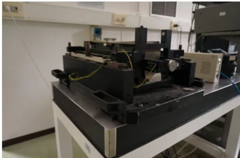
Figure 3.APS 113 ELECTRO-SEIS horizontal vibrating table.
2.4 Discussion of the methods
Table 1 summarizes some considerations concerning the spe-cific characteristics of the methods to be compared, in order to give information about the possibility of using them in-field, for the on-line andin-line calibration of MEMS, and about their capability of satisfying requirements involved in these applications.
2.5 Test bench and test procedure
For the comparison among calibration methods, two different accelerometers have been considered:
– a MEMS accelerometer (Sequoia FastTracer®) with a capacitive transduction system, with digital output to a computer, via a standard USB port. The output indicates the acceleration (nominal sensitivity of the order of 1, dimensionless);
– a piezo-electric accelerometer (PCB 356A15) with analogue output (nominal sensitivity of the order of 10 mV m−1s2).
The test bench used is a vibrating table with a horizontal linear slide, the APS 113 ELECTRO-SEIS shaker (Fig. 3). It is a long-stroke, electro-dynamic force generator specifi-cally suitable for low-frequency vibration testing. The slide is moved according to a sinusoidal law.
In Method 1 the accelerometer is fixed directly on the hor-izontal vibrating table, with one of the three axes parallel to the motion direction. All three axes are tested in this way, recursively.
In Method 2 and Method 3 an inclined steel clamp is fixed on the vibrating table; the inclination angle θ is 35◦ with respect to the horizontal plane (Fig. 4). The inclined steel clamp allows us to obtain a specified angleα(Method 2) or different angles α(Method 3). The motion of the vibrating table is accurately monitored by a laser Doppler vibrome-ter (LDV), as depicted in Fig. 4c.
The amplitude of the reference acceleration signal is ob-tained by applying Eq. (12),ωbeing the pulsation of the si-nusoidal motion andvvibthe velocity measured by the LDV.
aref=ω·vvib (12)
The data acquisition system (DAQ) used is the NI USB-4431 by National Instruments. The module consists of a single analogue output and four analogue input channels for read-ing (one is connected to the LDV and the other three to the outputs of the PCB accelerometer under test); each channel is equipped with antialiasing filters. The output channel drives the vibrating table. LabVIEW software is used for DAQ sig-nal acquisition.
2.6 Description of the experiments
Tests are carried out at the excitation frequencies of f1=
3 Hz andf2=6 Hz, at different amplitudes in the range 2 to
20 ms−2. Independent tests are carried out in two different configurations.
– Method 1: parallel excitation, with respect to the mea-suring axes of the accelerometer. The sensors are ex-cited along the main measuring componentsx, y and
zaxes, according to standards (ISO 16063-1, 1998; ISO 16063-11, 1999; ISO 16063-31, 2009).
– Method 2: inclined excitation with respect to the mea-suring axes of the accelerometer (θ=35◦,α=135◦). – Method 3: inclined excitation, with respect to the
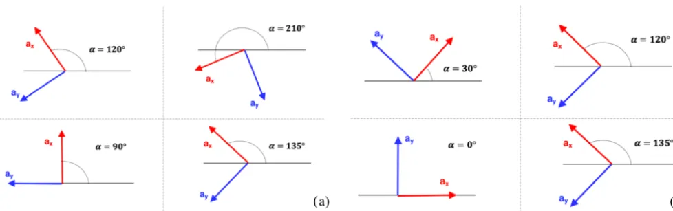
mea-suring axes of the accelerometer. Each sensor is rotated, according to four different angles,α, between thexaxis of the accelerometer and the horizontal. Depending on the specific sensor under test,αtakes the following val-ues: 0, 30, 90, 120, 135, and 210◦, as in Fig. 5.
2.7 Comparison between post-processing techniques In order to determine whether and to what extent the cali-bration methodologies are equivalent, the following results are compared, obtained through the application of the three above-mentioned methodologies:
– calibration tests of the same accelerometer, on the same test bench (high-performance linear slide);
– calibration tests of different accelerometers, of different technology and quality levels.
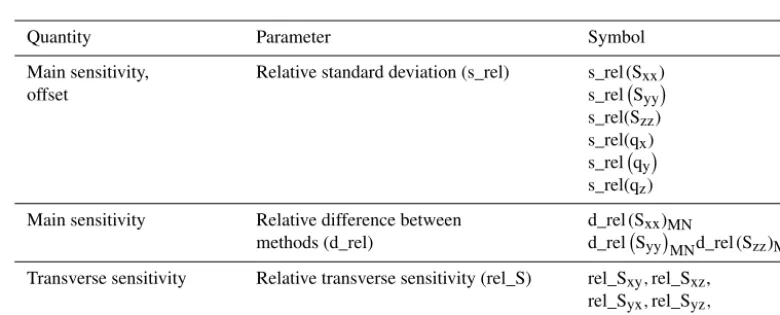
The comparison of the results and the assessment of the pos-sible equivalence between methods is made by the param-eters whose symbols are defined in Table 2, whereM and
N assume the following numbers: 1, 2, 3, depending on the specific method applied (e.g. d_rel(Sxx)MN, for M=3 and
N=2 stands for d_rel(Sxx)32, i.e. the relative difference
Figure 4.Particulars of the test bench: indication of the directions of acceleration. Piezo-electric(a)and MEMS(b)sensors, mounted on the inclined clamp. Laser vibrometer(c).
Table 2.Parameters used for the comparison.
Quantity Parameter Symbol
Main sensitivity, offset
Relative standard deviation (s_rel) s_rel (Sxx)
s_rel Syy
s_rel(Szz)
s_rel(qx)
s_rel qy
s_rel(qz)
Main sensitivity Relative difference between methods (d_rel)
d_rel (Sxx)MN
d_rel SyyMNd_rel (Szz)MN
Transverse sensitivity Relative transverse sensitivity (rel_S) rel_Sxy,rel_Sxz,
rel_Syx,rel_Syz,
rel_Szxrel_Szy
Details on the evaluation of each parameter are reported in Appendix A, taking as an example the main sensitivitySxx (i.e. the main sensitivity along the measuring x axis of the accelerometer).
In the following, the quantities used for comparison are summarized:
– the sensitivities and transverse sensitivities of each ac-celerometer and the related variability;
– the relative differences between methods of the main and the transverse sensitivities;
– sensitivities obtained by applying each method, taking into account the specific uncertainty.
3 Results
This section is organized as follows: Sects. 4.1 and 4.2 re-port the results obtained for the two accelerometers under test
(piezo-electric and MEMS), respectively. In each of them, the results of the three methods described are shown and a comparison among them is carried out.
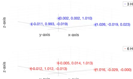
For the results obtained for the sensitivity matrix, a graph-ical representation in the 3-D space is used according to the scheme of Fig. 6. Each point represents a row of the sensitiv-ity matrix. The sensitivsensitiv-ity components are expressed in mil-livolt per metre second squared (mV m−1s2), for the
piezo-electric accelerometer, while they are dimensionless for the MEMS accelerometer, since the digital output values are di-rectly expressed in metres per second squared (m s−2).
Thexaxis represents the locus of the ideal response along the x axis itself of the three-axis accelerometer (Sxx6=0;
Figure 5.Angles of rotation of the accelerometers:(a)MEMS accelerometer;(b)piezo-electric accelerometer.
Table 3.Piezo-electric accelerometer: comparison between methods (%).
Frequency Methods d_rel (Sxx)MN d_rel SyyMN d_rel (Szz)MN
M=2;N=1 0.51 1.3 2.0
3 Hz M=3;N=1 −0.18 −0.24 0.91
M=3;N=2 −0.69 −1.5 −1.1
M=2;N=1 0.54 1.2 1.9
6 Hz M=3;N=1 −0.20 −1.1 −1.3
M=3;N=2 −0.74 −2.3 −3.2
Figure 6.3-D diagram for the sensitivity matrix: scheme and nota-tion.
3.1 Piezo-electric accelerometer
3.1.1 Method 1
Figure 7 represents the sensitivity matrix obtained by ap-plying Method 1, as described in Sect. 2.1, at 3 Hz (upper side) and 6 Hz (bottom side). The relative standard deviation (s_rel), defined in Table 1 and Appendix A, of all main sen-sitivities is negligible, being less than 0.03 %.
Figure 7.Piezo-electric accelerometer: sensitivity matrix obtained by means of Method 1 (3-D diagram).
3.1.2 Method 2
Table 4.MEMS accelerometer: comparison between methods (%).
Frequency Methods d_rel (Sxx)MN d_rel SyyMN d_rel (Szz)MN
M=2;N=1 0.73 −0.12 −0.19
3 Hz M=3;N=1 2.8 −0.49 1.1
M=3;N=2 2.1 −0.37 −0.93
M=2;N=1 0.68 −0.25 0.11
6 Hz M=3;N=1 1.8 1.5 1.4
M=3;N=2 1.1 1.7 1.3
Figure 8.Piezo-electric accelerometer: sensitivity matrix obtained by means of Method 2 (3-D diagram).
Figure 9.Piezo-electric accelerometer: sensitivity matrix obtained by means of Method 3 (3-D diagram).
3.1.3 Method 3
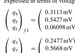
Figure 9 represents the sensitivity matrix obtained by ap-plying Method 3, as described in Sect. 2.3, at 3 Hz (upper side) and 6 Hz (bottom side). The relative standard devia-tion (s_rel) of all main sensitivities is negligible (less than 0.08 %). As a first approximation, the mean main sensitiv-ities appear coherent to those obtained through Method 1 (Fig. 7). The offset vectors atf1=3 Hz andf2=6 Hz are as
in the following, and they are considered negligible; there-fore, their variability is meaningless. For the piezo-electric accelerometer under investigation, the output values are in millivolt (mV), and as a consequence the offset values are
Figure 10. Piezo-electric accelerometer: comparison between methods (main sensitivity along thexaxis,Sxx).
expressed in terms of voltage.
qx
qy
qz
f1
=
0.3113 mV 0.5427 mV 0.06098 mV
;
qx
qy
qz
f2
=
0.2477 mV 0.5668 mV 0.5839 mV
.
3.1.4 Comparison between methods
Relative differences between methods (d_rel) obtained by applying the three methods are reported in Table 3, when the piezo-electric sensor is excited at 3 and 6 Hz, respectively.
Differences between Method 2 and Method 1 are al-ways positive up to 2 %. Differences between Method 3 and Method 1 are both negative and positive and in the range ±1.3 %. The highest differences arise between Method 3 and Method 2, being d_rel(Szz)32= −3.2 % (at 6 Hz).
Figures 10–12 highlight, for each axis, the relative posi-tion and differences among methods. Expanded uncertainty (k=2) of results, estimated according to D’Emilia et al. (2018), is also represented in Figs. 10–12 by error bars.
3.1.5 Reproducibility: transverse sensitivities
Figure 11. Piezo-electric accelerometer: comparison between methods (main sensitivity along theyaxis,Syy).
Figure 12. Piezo-electric accelerometer: comparison between methods (main sensitivity along thexaxis,Szz).
have been obtained by means of Method 1 and Method 3, which take these terms into account explicitly, and can be considered negligible in both cases.
3.2 MEMS accelerometer 3.2.1 Method 1
Figure 13 represents the sensitivity matrix obtained by ap-plying Method 1, as described in Sect. 2.1, at 3 Hz (upper side) and 6 Hz (bottom side). The relative standard deviation (s_rel), defined in Table 1 and Appendix A, of all main sen-sitivities is negligible (less than 0.02 %).
3.2.2 Method 2
Figure 14 represents the sensitivity matrix obtained by ap-plying Method 2, as described in Sect. 2.2, at 3 Hz (upper side) and 6 Hz (bottom side). Also in this case, the relative standard deviation (s_rel) appears negligible with respect to the mean sensitivities, which results in less than 0.09 %.
Figure 13.MEMS accelerometer: sensitivity matrix obtained by means of Method 1 (3-D diagram).
Figure 14.MEMS accelerometer: sensitivity matrix obtained by means of Method 2 (3-D diagram).
3.2.3 Method 3
Figure 15 represents the sensitivity matrix obtained by ap-plying Method 3, as described in Sect. 2.3, at 3 Hz (upper side) and 6 Hz (bottom side). The relative standard devia-tion (s_rel) of all main sensitivities is negligible (less than 0.06 %). The offset vectors atf1=3 Hz and f2=6 Hz are
as in the following.
qx values are not negligible at both frequencies. For the MEMS accelerometer under investigation, the digital output values are in metres per second squared (m s−2), and as a consequence the offset values are expressed in terms of ac-celeration.
qx
qy
qz
f1
=
0.3576 ms−2 −0.06304 ms−2 0.1650 ms−2
;
qx
qy
qz
f2
=
0.1662 ms−2 −0.07268 ms−2 0.1345 ms−2
.
3.2.4 Comparison between methods
Figure 15. MEMS accelerometer: sensitivity matrix obtained by means of Method 3 (3-D diagram).
Figure 16.MEMS accelerometer: comparison between methods (main sensitivity along thexaxis,Sxx).
the MEMS sensor is excited at 3 and 6 Hz. Figures 16–18 highlight the differences between methods in terms of the mean main sensitivities obtained.
Expanded uncertainties (k=2) of results, estimated ac-cording to D’Emilia et al. (2018), are also represented in Figs. 16–18 by error bars.
The differences of Method 3 with respect to Method 1 are higher than those of Method 2.
3.2.5 Reproducibility: transverse sensitivities
The relative transverse sensitivities (rel_S) for all axes ob-tained by means of Methods 1 and 3, which take these terms into account explicitly, are all under 4 %, and can be consid-ered negligible in both cases.
3.3 Discussion of the results
The highest differences of main sensitivity values between the indications of Method 1 and Method 3, of the order of 2 %, are associated with higher values of main sensitivity and offset uncertainty, as evaluated in Method 3. The ability to calculate together transverse sensitivities andQ=(qi) terms is a valuable capability, even though some interactions
be-Figure 17.MEMS accelerometer: comparison between methods (main sensitivity along theyaxis,Syy).
Figure 18.MEMS accelerometer: comparison between methods (main sensitivity along thexaxis,Szz).
tween them could appear, especially when static acceleration can be measured as in a MEMS accelerometer. No significant differences arise in the case of a piezo-electric accelerometer.
The main results are according to the following items:
– the methods offer reproducible results if differences be-tween them and the uncertainty of each method are taken into account;
– the uncertainty of Method 1, very close to the standard procedure, is very low, of the order of 0.5 %. Anyway, if the calibration procedure is considered, it is more com-plex and expensive than the other ones; furthermore, it seems not suitable for in-field application, with many of the procedure steps similar to a primary calibration;
applica-tions where transversal sensitivity effects could be rele-vant.
– The uncertainty of Method 3 is of the order of 3 %, that is, an intermediate behaviour, as for precision. It is in-tended to be capable of fitting in a satisfactory way most requirements for in-line and on-line calibration. This method allows the evaluation of transversal sensitivity and of offset terms; therefore, if these effects are re-markable, they can be estimated and do not affect the precision of the calibration.
4 Conclusions
The reproducibility of different methods for calibration of tri-axial accelerometers has been evaluated by means of a high-performance test bench, based on a linear slide and a high-accuracy laser Doppler vibrometer as a reference. The main sensitivities have been analysed and, where applicable, also transversal ones, in order to get information about the possibility of using new methods for theon-lineandin-line calibration of MEMS and about the capability of the methods of satisfying requirements involved in these applications, like low-cost calibration, operability, traceability and simplicity of procedures.
Two different accelerometers have been tested, a piezo-electric one and a MEMS one of capacitive type, different with reference to the ability to measure a constant accelera-tion.
The comparison refers to the following calibration proce-dures:
– Method 1, extending the indications of the standard to the case of a tri-axial accelerometer;
– Method 2, involving the simultaneous excitation of all three axes of the accelerometer under test, mounting it onto the surface of a clamp;
– Method 3, describing the relation between the input ac-celerations and the output signals in terms of the sensi-tivity matrixS=(Sij) and the offset vectorQ=(qi). A low-frequency range of vibration has been studied, 3 to 6 Hz, with amplitude of acceleration ranging from 2 to 20 ms−2, operated along one axis.
The methods offer reproducible results if differences be-tween them and the uncertainty of each method are taken into account, for both piezo-electric and MEMS accelerome-ters. Differences and extended uncertainty are of the order of a few percent.
Methods 2 and 3 appear suitable for in-field applications, even though some differences arise, in particular the follow-ing.
– Method 2 is quick and simple. Anyway, it does not al-low us to evaluate the transversal sensitivities and their
effect. This aspect strongly affects its uncertainty: if all the uncertainty contributions are considered, its relative uncertainty is of the order of 5 %. It is unsuitable for ap-plications where transversal sensitivity effects could be relevant.
– The uncertainty of Method 3 is of the order of 3 %, that is, generally satisfactory, as for precision. This method allows the evaluation of transversal sensitivity and of offset terms; therefore, if these effects are remarkable, they can be estimated and do not affect the precision of the calibration. It is able to fit in a satisfactory way most requirements forin-lineandon-line calibration and to compensate in a satisfactory manner most of the uncer-tainty causes in the calibration of tri-axial accelerome-ters.
Appendix A: Parameters used for the comparison
In the following, the parameters of Table A1 have been made more explicit. The equations referring toSxxare also applied to the main sensitivitiesSyyandSzzand to the offset vector,
qx,qy,qz(when Method 3 is taken into account).
It has to be pointed out that the variability of the results is evaluated on six entire cycles of oscillation (n=6 and the subscript kdenotes the kth cycle). For each accelerometer, for each kind of test, three repetitions are executed, in re-peatability conditions.
Table A1.Parameters used for the comparison: symbols and equations.
Quantity Parameter Symbols Equation
Main sensitivity Mean value S,q Sxx=1n
P
k
Sxxk
Offset Standard deviation SD SD (Sxx)=
s
P k
Sxx k−Sxx 2
n−1
Relative standard deviation s_rel s_rel (Sxx)=SD(SSxx) xx
·100
Mean sensitivities of method couples S Sxx12= Sxx1+2Sxx2
Sxx13= Sxx1+2Sxx3
Sxx23= Sxx2+2Sxx3
Main sensitivity Relative difference between methods d_rel d_rel(Sxx)21=Sxx2−Sxx1 Sxx12
·100
d_rel(Sxx)31=Sxx3−Sxx1 Sxx13
·100
d_rel(Sxx)32=Sxx3−Sxx2 Sxx23
·100
Transverse sensitivity Relative transverse sensitivity rel_S rel_Sxy=Sxy Sxx
·100;rel_Sxz= Sxz Sxx
·100;
rel_Syx= Syx Syy
·100;rel_Syz=Syz Syy
·100;
rel_Szx=Szx Szz
·100;rel_Szy=Szy Szz
Competing interests. The authors declare that they have no conflict of interest.
Edited by: Nam-Trung Nguyen Reviewed by: two anonymous referees
References
Batista, P., Silvestre, C., Oliveira, P., and Cardeira, B.: Ac-celerometer calibration and dynamic bias and gravity estimation: Analysis, design, and experimental evalua-tion, IEEE T. Control Syst. Technol., 19, 1128–1137, https://doi.org/10.1109/TCST.2010.2076321, 2011.
Borgia, E.: The Internet of Things vision: Key features, ap-plications and open issues, Comput. Commun., 54, 1–31, https://doi.org/10.1016/j.comcom.2014.09.008, 2014.
Chen, D. and Han, J.: Application of wavelet neural network in sig-nal processing of MEMS accelerometers, Microsyst. Technol., 17, 1–5, https://doi.org/10.1007/s00542-010-1169-7, 2011. Czech, K. R. and Gosk, W.: Measurement of surface vibration
ac-celerations propagated in the environment, Proc. Eng., 189, 45– 50, https://doi.org/10.1016/j.proeng.2017.05.008, 2017. D’Emilia, G., Gaspari, A., and Natale, E.:
Dy-namic calibration uncertainty of three-axis low fre-quency accelerometers, Acta IMEKO, 4, 75–81, https://doi.org/10.21014/acta_imeko.v4i4.239, 2015.
D’Emilia, G., Gaspari, A., and Natale, E.: Evalu-ation of aspects affecting measurement of three-axis accelerometers, Measurement, 77, 95–104, https://doi.org/10.1016/j.measurement.2015.08.031, 2016a. D’Emilia, G., Di Gasbarro, D., Gaspari, A., and Natale, E.:
Ac-curacy improvement in a calibration test bench for accelerom-eters by a vision system, Proc. Int. Conf. on Vibration Measure-ments by Laser and Noncontact Techniques: Advances and Ap-plications (Ancona), American Institute of Physics Inc., 1740, 090003, https://doi.org/10.1063/1.4952690, 2016b.
D’Emilia, G., Gaspari, A., Mazzoleni, F., Natale, E., and Schiavi, A.: Calibration of tri-axial MEMS accelerometers in the low-frequency range – Part 2: uncertainty assessment, submitted to J. Sens. Sens. Syst., 2018.
D’Emilia, G., Lucci, S., Natale, E., and Pizzicannella, F.: Validation of a Method for Composition Measurement of a Non-Standard Liquid Fuel for Emission Factor Evaluation, Measurement, 44, 18–23, https://doi.org/10.1016/j.measurement.2010.08.016, 2011.
Fong, W. T., Ong, S. K., and Nee, A. Y. C.: Methods for in-field user calibration of an inertial measurement unit with-out external equipment, Meas. Sci. Technol., 19, 085202, https://doi.org/10.1088/0957-0233/19/8/085202, 2008.
Frosio, I., Pedersini, F., and Borghese, N. A.: Autocalibration of MEMS Accelerometers, IEEE Trans. Instrum. Meas., 58, 2034– 2041, https://doi.org/10.1109/TIM.2008.2006137, 2009. Frosio, I., Pedersini, F., and Borghese, N. A.:
Autocali-bration of triaxial MEMS accelerometers with automatic sensor model selection, IEEE Sens. J., 12, 2100–2108, https://doi.org/10.1109/JSEN.2012.2182991, 2012.
Geist, J. C., Afridi, M. Y., McGray, C., and Gaitan, M.: Gravity-Based Characterization of Three-Axis Accelerometers in Terms of Intrinsic Accelerometer Parameters, J. Res. Natl. Inst. Stand. Technol., 122, 1–14, https://doi.org/10.6028/jres.122.032, 2017. Griffin, M. J.: 2014 Handbook of human vibration, St. Louis:
Else-vier Science, 2014.
Glueck, M., Buhmann, A., and Manoli, Y.: Autocalibration of MEMS accelerometers, Proc. Int. Conf. on Instrumenta-tion and Measurement Technology (Graz) (IEEE), 1788–1793, https://doi.org/10.1109/I2MTC.2012.6229157, 2012.
Halim, M. A. and Park, J. Y.: A frequency up-converted elec-tromagnetic energy harvester using human hand-shaking, J. Phys. Conf. Ser., 476, 012119, https://doi.org/10.1088/1742-6596/476/1/012119, 2013.
ISO 16063-1:1998 – Methods for the calibration of vibration and shock transducers – Part 1: Basic concepts, 1998.
ISO 16063-11:1999 – Methods for the calibration of vibration and shock transducers – Part 11: Primary vibration calibration by laser interferometry, 1999.
ISO 16063-21:2003 – Methods for the calibration of vibration and shock transducers – Part 21: Vibration calibration to a reference transducer, 2003.
ISO 16063-31:2009 – Methods for the calibration of vibration and shock transducers – Part 31: Testing of transverse vibration sen-sitivity, 2009.
Rainieri, C., Fabbrocino, G., and Verderame, G. M.: Non-destructive characterization and dynamic iden-tification of a modern heritage building for service-ability seismic analyses, NDT and E Int., 60, 17–31, https://doi.org/10.1016/j.ndteint.2013.06.003, 2013.
Ripper, G. P., Ferreira, C. D., Dias, R. S., and Micheli, G. B.: Improvement of the primary low-frequency accelerometer cal-ibration system at INMETRO, IMEKO 4th TC22 Int. Conf., Helsinki, 2017.
Rohac, J., Sipos, M., and Simanek, J.: Calibration of low-cost triaxial inertial sensors, IEEE Instr. Meas. Mag., 18, 32–38, doi10.1109/MIM.2015.7335836, 2015.
Sabato, A., Niezrecki, C., and Fortino, G.: Wireless MEMS-based accelerometer sensor boards for structural vibra-tion monitoring: a review, IEEE Sens. J., 17, 226–235, https://doi.org/10.1109/JSEN.2016.2630008, 2017.
Schiavi, A., Mazzoleni, F., and Germak, A.: Simultaneous 3-axis mems accelerometer primary calibration: descrip-tion of the test-rig and measurements, Proc. XXI IMEKO World Congress on Measurement in Research and Indus-try, Prague, 30 August–4 September 2015, 1, 2161–2164, https://doi.org/10.13140/RG.2.1.1049.4487, 2015.