On p-generalized elliptical random processes

R E S E A R C H

Open Access

On

p

-generalized elliptical random

processes

Klaus Müller and Wolf-Dieter Richter

*Correspondence:

[email protected]

University of Rostock, Institute of Mathematics, Ulmenstraße 69, Rostock, Germany

Abstract

We introduce rank-k-continuous axis-alignedp-generalized elliptically contoured distributions and study their properties such as stochastic representations, moments, and density-like representations. Applying the Kolmogorov existence theorem, we prove the existence of random processes having axis-alignedp-generalized elliptically contoured finite dimensional distributions with arbitrary location and scale functions and a consistent sequence of density generators ofp-generalized spherical invariant distributions. Particularly, we consider scale mixtures of rank-k-continuous axis-aligned p-generalized elliptically contoured Gaussian distributions and answer the question when ann-dimensional rank-k-continuous axis-alignedp-generalized elliptically contoured distribution is representable as a scale mixture ofn-dimensional rank-k-continuous

p-generalized Gaussian distribution for a suitable mixture distribution of a positive random variable. Based on this class of multivariate probability distributions, we introduce scale mixedp-generalized Gaussian processes having axis-aligned finite dimensional distributions beingp-generalizations of elliptical random processes. Additionally, some of their characteristic properties are discussed and approximates of trajectories of several examples such asp-generalized Student-tandp-generalized Slash processes having axis-aligned finite dimensional distributions are simulated with the help of algorithms to simulate rank-k-continuous axis-alignedp-generalized elliptically contoured distributions.

Keywords: Axis-alignedp-generalized elliptically contoured distributions, Density-like representation, Kolmogorov consistency conditions,p-generalized spherically invariant random processes, Scale mixtures of multivariate axis-alignedp-generalized elliptically contoured Gaussian distributions, Simulation

1 Introduction

Random processes may be constructed and characterized in different ways. Apart from constructions via families of random variables whose members satisfy, e.g., specific autoregressive relations or are coefficients of specific series representations, the existence of random processes can be studied following the fundamental existence theorem due to

Kolmogorov (1933). The explicit knowledge of the family of finite dimensional

distribu-tions (fdds) can be used then to establish some of the properties of the random process by proving corresponding ones of the fdds. Basic technical problems to be solved this way belong to multivariate distribution theory. In the present paper, Kolmogorov’s theorem is used to prove the existence of real valued random processes having axis-aligned

p-generalized elliptically contoured (apec) fdds, thus beingp-generalizations of elliptical

random processes having axis-aligned fdds.

Well studied examples of random processes which can be constructed via Kolmogorov’s existence theorem are real valued Gaussian processes with emphasis on the

Brown-ian motion, see Shiryaev (1996) and Schilling and Partzsch (2014). Apart from further

examples as random processes with independent values, random processes with inde-pendent increments as well as Markov processes, spherically invariant random processes being also known as elliptical random processes can be constructed this way. The latter

are introduced in Vershik (1964) as random processes consisting of quadratically

inte-grable random variables such that if two of them have the same variance, they follow the same distribution. Corresponding characteristic functions and densities are determined

in Blake and Thomas (1968). Yao (1973) and Kano (1994) characterize spherically

invari-ant random processes by establishing that their families of fdds are what is called now scale mixtures of Gaussian distributions having one and the same mixture distribution.

The notion of a scale mixture but is first introduced in Andrews and Mallows (1974)

and, independently, Wise and jun Gallagher (1978) show that an elliptical random

pro-cess can be represented as a product of a Gaussian propro-cess and a positive random variable

being independent of it. Additionally, in Huang and Cambanis (1979), the structure of

the space of all second order spherically invariant random processes is studied and used to solve nonlinear estimation problems. Finally, based on the concepts of expansive and semi-expansive sequences of elliptically contoured distributions and apart from analogue

representation theorems in Yao (1973) and Kano (1994), a formula to determine the

cor-responding mixture distribution of the family of fdds of a spherically invariant random

process is determined in Gómez-Sánchez-Manzano et al. (2006).

Besides a thematically assorted summary of several articles on the theory of spherically invariant random processes, numerous applications of these random processes such as modelings of bandlimited speech waveform, of radar clutters, of radio propagation

dis-turbances and of equalization and array processing are dealt with in Yao (2003). Furthermore,

the author discusses simulations of trajectories of spherically invariant random processes

based on the work in Brehm and Stammler (1987), Conte et al. (1991), and Rangaswamy

et al. (1995). More recent applications deal with fading models from spherically

invari-ant random processes in Biglieri et al. (2015) and with MIMO radar target

localiza-tion and performance evalualocaliza-tion under spherically invariant random process clutter in Zhang et al. (2017).

The notion of a scale mixture of Gaussian distributions is introduced in Andrews

and Mallows (1974) as the distribution of the product of a Gaussian variable and

an independent positive random variable. A multivariate generalization is given in

Lange and Sinsheimer (1993). Using numerous equivalent definitions, scale

mix-tures of Gaussian distributions are also studied in West (1987), Gneiting (1997),

Eltoft et al. (2006), Gómez-Sánchez-Manzano et al. (2006, 2008), and Hashorva

(2012). According to Andrews and Mallows (1974), Lange and Sinsheimer (1993), and

Gómez-Sánchez-Manzano et al. (2006), scale mixtures of Gaussian distributions

Applications of scale mixtures of Gaussian distributions are given in the fields of

nat-ural images, insurances and quantitative genetic in Wainwright and Simoncelli (2000),

Choy and Chan (2003), and Gómez-Sánchez-Manzano et al. (2008). More recent

appli-cations are Gaussian scale mixture models for robust multivariate linear regression with

missing data in Ala-Luhtala and Piché (2016), testing homogeneity in a scale mixture of

Gaussian distributions in Niu et al. (2016), and adaptive robust regression with

continu-ous Gaussian scale mixture errors in Seo et al. (2017).

For any choice ofp > 0, introducing the notion of a p-generalization of a

spher-ically invariant random process means the transition from spherspher-ically contoured to

ln,p-symmetric fdds, the transition from regular elliptically contoured to suitably

intro-duced p-generalized elliptically contoured distributions and the associated

consider-ation of suitable non-Euclidean instead of Euclidean geometries, respectively. To be

more specific, a well-known example is the n-dimensional p-generalized (spherical)

Gaussian distribution being introduced already in Subbotin (1923) and having the

probability density function (pdf )

f(x)= ⎛ ⎝ p1−

1 p

2

1

p

⎞ ⎠ n

exp

−1

p n

i=1 |xi|p

, x=(x1,. . .,xn)T∈Rn,

andp-generalized Weibull, Pearson type II and Pearson type VII distributions are dealt

with in Gupta and Song (1997). Additionally, ap-generalized spherical coordinate

trans-formation, ap-generalized surface content measure as well as numerousp-generalized

probability distributions and statistics such asp-generalized versions of theχ2-, Student

and Fisher distributions are considered in Richter (2007); Richter (2009).

The more general class of continuous ln,p-symmetric distributions is studied in

Arellano-Valle and Richter (2012), Kalke and Richter (2013), Müller and Richter (2016a,

b,2017a,b) as well as several references given there. In the present paper, we introduce a class of multivariate apec distributions containing both regular and singular

distribu-tions and covering the classes of continuousln,p-symmetric and common axis-aligned

elliptically contoured distributions.

For a nonempty index setI⊆R, a Polish space(E,ρ)and a familyQof probability

mea-sures on the product spacesEJ,BJfor nonempty finite subsetsJ⊆Iand the Borel sigma

fieldBonE with respect toρ, ifQis projective onE, Kolmogorov’s existence theorem

states the existence of a random process having time setIand state spaceEsuch that its

family of fdds is equal toQ. The projectivity ofQonEcan be shown by checking the

con-sistency conditions in Kolmogorov (1956). This will be discussed for the particular case

E = Rin “Sketch of proof” section. This way, we prove the existence of real valued

ran-dom processes having apec fdds. Such ranran-dom processes arep-generalizations of elliptical

random processes having axis-aligned fdds. Moreover, for the special case of scale mixed

p-generalized Gaussian processes having axis-aligned fdds, basic properties such as

thepth root function, is completely monotone and secondly that the corresponding mix-ture distribution is in a well defined way closely connected to the inverse Laplace-Stieltjes transform of this composition.

The paper is structured as follows. In “The class ofn-dimensional rank-k-continuous

axis-aligned p-generalized elliptically contoured distributions” section, n-dimensional

apec distributions are introduced as location-scale generalizations of continuous ln,p

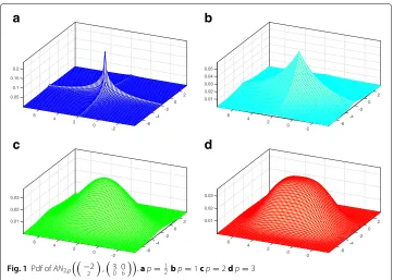
-symmetric distributions, and some of their properties such as stochastic representations, moments and pdf-like representations are discussed. Furthermore, the pdfs of bivariate

p-generalized spherical as well as of bivariate apec Gaussian distributions are visualized

for several values of p > 0. Our main result on the existence ofp-generalizations of

elliptical random processes is presented in “Main result” section. A sketch of its proof

consisting of four basic steps is given in “Sketch of proof” section, and an approximate

simulation of the trajectories of the new random processes is discussed in “Simulation”

section. Examples illustrating the developed theory are studied in the fourth section. In “Scale mixtures of apec Gaussian distributions” section, scale mixtures of multivariate apec Gaussian distributions are introduced and some of their characteristic properties such as stochastic representations, moments, specific conditional distributions, and their connections to completely monotone functions are discussed. Random processes whose families of fdds are families of scale mixtures of multivariate apec Gaussian distributions with one and the same mixture distribution as well as some of their basic properties

are studied in “Scale mixedp-generalized Gaussian processes having axis-aligned fdds”

section. All proofs are given in “Proofs” section. For the sake of a better readability, the

proofs of certain results are prepared by proving certain particular cases first. An algo-rithm to simulate arbitrary apec distributions and another one to particularly simulate scale mixtures of apec Gaussian distributions with an explicitly known mixture

distribu-tion are presented in Appendix7.1. The latter one is used in Appendix7.2to simulate

approximations of trajectories ofp-generalized Student-tas well asp-generalized Slash

processes having axis-aligned fdds. Finally, we remark that all figures presented here are made using the program MATLAB.

2 The class ofn-dimensional rank-k-continuous axis-alignedp-generalized elliptically contoured distributions

For eachp > 0 andn ∈ N, we denote thep-functional inRn by|x|p =

_n

i=1

|xi|p 1

p ,

x = (x1,. . .,xn)T ∈ Rn, and theln,p-generalized surface content of theln,p-unit sphere Sn,p= {x∈Rn:|x|p=1}byωn,p,

ωn,p=

21_pn

pn−1n p

.

Furthermore, a functiong: [ 0,∞)→[ 0,∞)satisfying 0<In(g) <∞is called a

den-sity generating function of ann-variate distribution whereIn(g) =

∞

0

rn−1g(r)dr. An

n-dimensional random vectorX:→Rnon a probability space(,A,P)having the pdf

g|x|p

ωn,pIn(g),x∈R

n_{, is called continuousl}

n,p-symmetrically distributed with density

satisfyingIn(g) = _ω1

n,p is called a density generator (dg) and denoted byg

(n,p)_{. The pdf}

of the continuousln,p-symmetric distribution with dgg(n,p) isg(n,p)

|x|_p,x ∈ Rn, and

the corresponding probability law is denoted by_g(n,p). With a view to the special cases

listed below,_g(n,p)may also be calledn-dimensional continuousp-generalized spherical

distribution with dgg(n,p)_.

A well-known example of the latter type of probability distributions is the n

-dimensionalp-generalized (spherical) Gaussian distributionNn,p=_g(n,p)

PE where

g_PE(n,p)(r)= ⎛ ⎝ p1−

1 p

2

1

p

⎞ ⎠ n

exp

−1

pr p

, r≥0.

For visualizations of the pdf of this distribution forn ∈ {1, 2}and severalp > 0, we

refer to Kalke and Richter (2013) and Müller and Richter (2015). The class of continuous

ln,2-symmetric distributions coincides with the class of n-variate continuous spherical

distributions andNn,2 is then-dimensional standard Gaussian distribution. Numerous

properties such as stochastic representations, moments, and marginal distributions and

several types of dgs are discussed in Gupta and Song (1997), Richter (2009), Arellano-Valle

and Richter (2012), and Müller and Richter (2016a).

Letμ ∈ Rnbe a constant vector andD = diag(d1,. . .,dn)ann×ndiagonal matrix

having nonnegative diagonal entries and positive rank rk() = k. Moreover, letI1 =

{i1,. . .,ik} ⊆ {1,. . .,n}with|I1| =kandi1<i2< . . . <ikbe the set of indices such that di>0 ifi∈I1anddi=0 ifi∈I2= {1,. . .,n}\I1. Lete(n)i denote theith unit vector inRn

0n×nthen×nzero matrix,S1= diag

di1,. . .,dik

∈Rk×k_,W

1=

e(n)_i1 · · ·e(n)_i

k

∈Rn×k andW2∈Rn×(n−k)a matrix having columnse(n)i for alli∈I2, then,

W₁TDW1=S1 and W2TDW2=0(n−k)×(n−k).

Let√S1 = diag

di1,. . .,

dik

. The distribution of a random vectorXsatisfying

the stochastic representation

X=d μ+W1

S1Y whereY ∼g(k,p) (1)

is called ann-dimensional rank-k-continuous axis-alignedp-generalized elliptically

con-toured (kapec) distribution with location parameterμ, scaling matrixDand dgg(k,p)and

is denoted byAECn,p

μ,D,g(k,p). For simplicity, the distribution of such random vector

Xis just called apec distribution if its continuity and dimension as well as the rank of the

diagonal matrix parameterDare contextually clear or play only a minor role.

Here and in what follows,X =d ZandX ∼ mean that the random vectorsXandZ

follow the same distribution law and that the random vectorXfollows the distribution

lawL(X)= , respectively. In particular, for the special choice ofμandDto be the zero

vector 0nand identity matrixIn×ninRn, respectively, we haveAECn,p

0n,In×n,g(n,p)

=

g(n,p). For the special case ofp=2, the class ofAECn,2

μ,D,g(k,2)-distributions is

iden-tical with the class of commonn-variate axis-aligned elliptically contoured distributions.

Furthermore,AECn,p

μ,D,g_PE(k,p) is calledn-dimensional kapec Gaussian distribution

and is denoted ANn,p(μ,D). The family of apec distributions with full rank scaling

matrices as well as their star-shaped extensions and certain aspects of their inferential

Because of relation (1), a stochastic representation and properties of moments of n

-dimensional kapec distributions stated in Lemmata2.1and2.2follow immediately from

corresponding results oflk,p-symmetric distributions in Richter (2009) and Arellano-Valle

and Richter (2012).

Lemma 2.1Let X ∼AECn,p

μ,D,g(k,p)whererk(D) = k. Then, the random vector X satisfies the stochastic representation

X=d μ+R·W1

S1Up(k)

where the random vector Up(k)is k-dimensional p-generalized uniformly distributed on Sk,p, R and Up(k)are stochastically independent and R is a nonnegative random variable with pdf

fR(r)=ωk,prk−1g(k,p)(r)1[0,∞)(r), r∈R.

Lemma 2.2 Let X ∼ AECn,p

μ,D,g(k,p) where rk(D) = k. Then, E(X) = μ if Ik+1g(k,p)is finite andCov(X) = σ_g2(k,p)D if Ik+2g(k,p)is finite where the univariate

variance component σ_g2_(k,p) of _g(k,p) satisfies σ_g2_(k,p) = 3

p

k p

1 p

k+2 p

_ωk,pIk+2(g(k,p)). The

components of X are independent if and only if g(k,p)=g_PE(k,p).

The justification for callingσ_g2(n,p) the univariate variance component ofg(n,p) is given

by the following lemma withk = 1. Examples ofσ_g2_(n,p) are given in Müller and Richter

(2016b). Let us remark that, according to Arellano-Valle and Richter (2012), for k = 1,. . .,n−1, the marginal dgg_(n)(k,p)of an arbitraryk-dimensional marginal distribution of

g(n,p)is

g_(n)(k,p)(r)= ωn−k,p p

∞

rp

y−rpn−kp −1_g(n,p)√p_{ydy, r}∈_{[ 0,}∞)_,

where the variability of the choice of the k marginal variables is established by the

permutation invariance of_g(n,p), see Müller and Richter (2016b).

Lemma 2.3For k=1,. . .,n−1,

σ2

g₍(k,pn))=σ 2

g(n,p).

DenotingM∗_n =[ 0,π)×(n−2)×[ 0, 2π)andMn =[ 0,∞)×M∗n forn ≥ 2, let theln,p

-spherical coordinate transformationSPHp(n):Mn → Rnbe defined as in Richter (2007).

Note thatSPHp(n) is bijective a.e. inMn and its inverse mapping as well as its Jacobian

are explicitly known. The next lemma combines and states more precisely some earlier results and introduces a second stochastic representation of random vectors following the distributionAECn,p

μ,D,g(k,p).

Lemma 2.4Let X ∼AECn,p

μ,D,g(k,p)whererk(D) = k. Then, the random vector X satisfies the stochastic representation

X=d μ+W1

S1·SPHp(k)

where the nonnegative random variables R, 1,. . ., k−1are mutually stochastic indepen-dent having pdfs

fR(r)=ωk,prk−1g(k,p)(r)1[0,∞)(r), r∈R,

f i(ψi)= ωk−i,p

ωk−i+1,p

(sin(ψi))k−i−1

Np(ψi)

k−i+11[0,π)(ψi), ψi∈R,i=1,. . .,k−2,

f _k−1(ψk−1)= _ω1 2,p

1

Np(ψk−1)2

1[0,2π)(ψk−1), ψk−1∈R.

Here, Np(ψ)=

|sin(ψ)|p+ |cos(ψ)|p1/pand fZdenotes the pdf of Z.

While the distributionAECn,p

μ,D,g(n,p) is regular and has a pdf, the distribution AECn,p

μ,D,g(k,p)_{is singular if rk(D) = k < nand may be characterized by a}

pdf-like representation as it was done in Khatri (1968) and Rao (1973, pp. 527-528) in case

of singular normal distributions and in Arellano-Valle and Azzalini (2006, Appendix

C) in case of singular unified skew-normal distributions. To this end, let U_WT

2(μ) =

{x ∈ Rn: WT

2x = W2Tμ} be ak-dimensional affine subspace inRn and λ(k)U_WT

2(μ) the

k-dimensional Lebesgue measure defined onU_WT

2(μ).

Lemma 2.5Let X ∼ AECn,p

μ,D,g(k,p)whererk(D) = k. Then, the distribution of X has pdf-like representation

1

di₁·. . .·dik

g(k,p)

S1 −1

W₁T(x−μ) p

, x∈Rn, (2)

and

W₂TX=W₂Tμ P−a.s. (3)

where the function given in (2) is interpreted as pdf in the space U_VT

2(μ)in which the whole

probability mass of X is concentrated according to Eq.3.

Lemma 2.5 can be read as follows. For X ∼ AECn,p

μ,D,g(k,p)_{, the orthogonal}

projectionY =U_WT

2(μ)(

X)ofXinto the subspaceU_WT

2(μ), and any eventB∈B

n_,

P(X∈B)=PY ∈B∩U_WT 2(μ)

= 1

di1·. . .·dik

B g(k,p)

S1

−1

WT

1(x−μ)_p

λ(k)_U WT

2(μ)

(dx) (4)

meaning that the probability measure induced by the random vector X, PX =

AECn,p

μ,D,g(k,p)_{, is absolutely continuous with respect to λ}(k)

U_VT 2(μ)

. Thus, (2) is the

Radon-Nikodym derivative ofPX _{with respect to the Lebesgue measureλ}(k)

U_VT 2(μ)

on the

subspaceU_WT

2(μ)ofR

n_{. Because of (4),g}(k,p) _{might be called density-like generator of}

AECn,p

μ,D,g(k,p)_{ifk < n. In particular, if rk(D)= n, thenW}

1 = In×nandW2is not

defined. Hence, Eq.3is not applicable and the function in (2) is the common pdf of the

distributionAECn,pμ,D,g(n,p). An example is illustrated in Fig.1.

At the end of this section, our consideration will be slightly extended in order to cover

the casek= rk(D)=0 or, equivalently,D=0n×n. To this end,AECn,p

μ, 0n×n,g(0,p)

2 0 -2 -4 -6 -2 0 2 4 6 0.05

0.1 0.15 0.2

2 0 -2 -4 -6 -2 0 2 4 6 0.05

0.02 0.01 0.04 0.03

2 0 -2 -4 -6 -2 0 2 4 6 0.01 0.02 0.03

2 0 -2 -4 -6 -2 0 2 4 6 0.01 0.02 0.03

a

b

c

d

Fig. 1Pdf ofAN2,p

−2 2

,3₀ 0₆.ap= ₂1bp=1cp=2dp=3

defined to be the Dirac distribution atμ ∈ Rn whereg(0,p)is just a symbol to maintain

previous notations.

While each finite dimensional distribution (fdd) of an elliptical process is elliptically contoured, in the next section the existence of random processes will be shown whose families of fdds consist of apec distributions.

3 Generalized elliptical random processes

3.1 Main result

In order to state our main result, we call a sequenceg(p)=g(k,p)

k∈Nof dgs of continuous

lk,p-symmetric distributions consistent if the following condition is satisfied for anyk∈N

and almost all(x1,. . .,xk)T∈Rk,

∞

−∞

g(k+1,p)

x1,. . .,xk,xk+1 T

p

dxk+1=g(k,p)

(x1,. . .,xk)T_p

. (5)

For the particular case of this definition ifp = 2, we refer to Kano (1994). Moreover,

for any nonempty subsetI ofR, any functionsm: I → RandS:I →[ 0,∞), and any

sequence g(p) = g(k,p)_k∈N of dgs of continuous lk,p-symmetric distributions, let the

family

n∈N

{t1,...,tn}⊆I

|{t1,...,tn}|=n

AECn,p

μ,D,g(k,p):μ=(m(t1),. . .,m(tn))T,

D= diag(S(t1),. . .,S(tn)),k=rk(D)

of apec distributions having dgs from g(p) and location and scale functions m andS,

respectively, be denoted byAECI_g(p)(m,S). Note that strict positivity ofSyields a family

AECI

be nonnegative, the familyAECI_g(p)(m,S)consists both of regular and singular

distribu-tions. In particular, the univariate member of this family corresponding tot∈Isuch that

S(t)=0 isAEC1,p

m(t), 0,g(0,p), i.e. an univariate kapec distribution withk=0.

Theorem 4.1If g(p)is consistent, thenAECI_g(p)(m,S)is projective onR.

Corollary 3.1According to the Kolmogorov existence theorem, for any nonempty subset I ofR, functions m:I →Rand S: I→[ 0,∞), and consistent sequence g(p), Theorem4.1

yields the existence of a real-valued random process havingAECI_g(p)(m,S)as its family of fdds.

A random process defined according to Theorem4.1and Corollary3.1is called random

process having apec fdds with location and scale functions mandS, respectively, and

sequenceg(p)of dgs of continuouslk,p-symmetric distributions. Such random process is

denoted byAECPp

m,S;g(p).

3.2 Sketch of proof

Because of the complexity of the proof of Theorem4.1, we first give a sketch of its

prin-cipal ideas. For the outline of details of proof, we refer to “Proof of Theorem 4.1” section.

The first step and fundamental argument to prove Theorem4.1and thus the existence of

the random processes according to Corollary3.1is to show that the familyAECI_g(p)(m,S) satisfies Kolmogorov’s consistency conditions. Let the set of all finite and nonempty sub-sets ofIbe denoted byH(I),H(I)= {J⊆I:J= ∅,|J|<∞}. According to Kolmogorov

(1956), a familyQ = QJ

{J∈H(I)} of probability measures on

R|J|_,B|J|_{,J ∈ H(I), is}

projective onRif the following two conditions are satisfied:

1) For allt1,. . .,tn,tn+1∈Ibeing pairwise distinct andA(n)∈Bn,

Q{t1,...,tn,tn+1}

A(n)×E

=Q{t1,...,tn}

A(n)

. (6)

2) For allt1,. . .,tn∈I,A(n)∈Bnbeing pairwise distinct and every permutationπof {1,. . .,n},

Q{t1,...,tn}

A(n)=Q{tπ(1),...,tπ(n)}

A(n)_π (7)

whereA(n)π =(xπ(1),. . .,xπ(n))T: (x1,. . .,xn)T∈A(n)

.

These two conditions are traditionally formulated using the notion of ordered sets which are assumed to have different elements, i.e. the sets{t1,t2}and{t2,t1}differ from

each other ift1 =t2, whereas (7) is not required in case of considering unordered sets,

see Shiryaev (1996, p. 168).

Condition (6) ensures that specific marginal distributions of elements of the familyQ

are elements of this family, too. Proving (6) for the family given in Theorem4.1will be

done in steps two and three. Since both of them are connected with transitions from joint to marginal distributions, we will use the notion of marginal dgsg_(k)(m,p),m=1,. . .,k−1,

according to “The class ofn-dimensional rank-k-continuous axis-alignedp-generalized

elliptically contoured distributions” section. Additionally, letg_(k)(k,p)=g(k,p)_{. Making use of}

Lemma 3.1A sequence g(p) = g(k,p)_k∈Nof dgs of continuous lk,p-symmetric distribu-tions is consistent if and only if for any k∈N

g_(k(k₊₁,p)₎=g(k,p) a.e. in[ 0,∞).

As a consequence, a sequenceg(p) of dgs of continuouslk,p-symmetric distributions

is consistent if and only if for any k ∈ Nthe marginal dgg_(k(k₊₁,p)₎ corresponding to the

(k+1)th elementg(k+1,p)ofg(p)coincides with thekth elementg(k,p). In the third step,

form≤n,m-dimensional marginal distributions ofn-dimensional apec distributions are

shown to bem-dimensional apec distributions with suitably modified vector and matrix

parameters and transitions to marginal dgs.

Lemma 3.2Forμ=(μ1,. . .,μn)T∈Rnand D= diag(d1,. . .,dn)having nonnegative

diagonal entries and rank k ≥ 0, let X = (X1,. . .,Xn)T ∼ AECn,pμ,D,g(k,p). Further, let m ∈ Nwith m ≤ n, J = {j1,. . .,jm} ⊆ {1,. . .,n}with j1 < . . . < jm, and XJ =

Xj1,. . .,Xjm T

the corresponding m-dimensional subvector of X. Then,

XJ ∼AECm,p

μJ,DJ,g_(k)(kJ,p)

whereμJ =

μj1,. . .,μjm T

, DJ = diagdj₁,. . .,djm

, and kJ =rk(DJ)≥0.

In the final step four, condition (7) ensures that the considered family of probability

distributions is big enough in a suitable sense. Its proof in case ofQ = AECI_g(p)(m,S)is based on the next lemma on distributions of specific linear transformations of random vectors following an apec distribution.

Lemma 3.3Let X ∼ AECn,p

μ,D,g(k,p)withrk(D) = k ≥ 0. Then, for every(n× n)-permutation matrix M and every b∈Rn,

L(MX+b)=AECn,p

Mμ+b,MDMT_,g(k,p)_.

These sketched four steps to prove Theorem 4.1are outlined in detail in “Proof of

Theorem 4.1” section in reverse order. At the end of the present section, we consider an

example of random processes being defined by Theorem4.1and Corollary3.1. More

gen-eral examples are studied in “Scale mixtures and particularp-generalizations of elliptical

random processes” section.

Example 3.1 Let g_PE(p) =

g_PE(k,p)

k∈N be the sequence of all dgs of multivariate p-generalized Gaussian distributions. Then, the consistency of g_PE(p)is immediately seen and for any nonempty subset I of R and any functions m: I → R and S: I →[ 0,∞), Theorem 4.1yields the existence of the real-valued random process AGPp(m,S)having

AECI

g(_PEp)(m,S)as its family of fdds. Such stochastic process is called p-generalized Gaussian process having axis-aligned fdds.

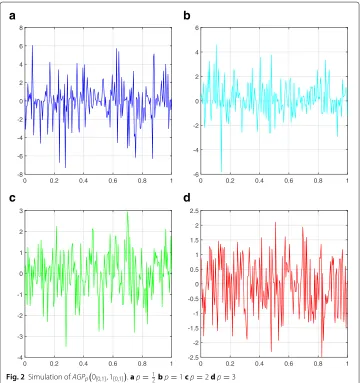
3.3 Simulation

In order to simulate a random processXhaving apec fdds, we considerI =[ 0, 1],

simu-late the marginal vector ofXregarding to the equidistant partition₂₀₀i :i=0,. . ., 200

of [ 0, 1] to get a realization of the random vector

X0,X 1

200,. . .,X199200,X1 T

connect the components of this realization in ascending order by linear functions to get

an approximate realization of a trajectory ofX. Since components of apec Gaussian

dis-tributed random vectors are independent, simulation of the random processAGPp(m,S)

according to the method described above is just the simulation of 201 univariate

p-generalized Gaussian variables having specific location and scale parameters. We

denote functions on [ 0, 1] taking constant values 0 and 1 by 0[0,1] and 1[0,1],

respec-tively. Results of the simulation of the random processAGPp

0[0,1], 1[0,1]

are shown for p∈1₂, 1, 2, 3in Fig.2. Note that scales of axes are highly dependent on the value ofp, but

also on the specific realization of a trajectory of the process. Moreover, in Fig.3, the effect

different location and scale functions mandS have on simulations of AGP3(m,S) are

shown. See also Appendix7.2for several other simulations of random processes having

apec fdds.

4 Scale mixtures and particularp-generalizations of elliptical random processes

4.1 Scale mixtures of apec Gaussian distributions

Let beμ ∈Rn,D ∈ Rn×na diagonal matrix having nonnegative diagonal elements and

rankk ≥ 0,V a positive random variable, andZ ∼ ANn,p(0n,D) independent ofV.

0 0.2 0.4 0.6 0.8 1 -8

-6 -4 -2 0 2 4 6 8

0 0.2 0.4 0.6 0.8 1 -6

-4 -2 0 2 4 6

0 0.2 0.4 0.6 0.8 1 -4

-3 -2 -1 0 1 2 3

0 0.2 0.4 0.6 0.8 1 -2.5

-2 -1.5 -1 -0.5 0 0.5 1 1.5 2 2.5

a

b

c

d

0 0.2 0.4 0.6 0.8 1 -2

-1 0 1 2 3 4 5 6 7 8

m

1

m

2

m

3

0 0.2 0.4 0.6 0.8 1 -3

-2 -1 0 1 2 3 4 5

0 0.2 0.4 0.6 0.8 1 -3

-2 -1 0 1 2 3 4

0 0.2 0.4 0.6 0.8 1 -1

0 1 2 3 4 5 6 7 8 9

0 0.2 0.4 0.6 0.8 1 0

0.2 0.4 0.6 0.8 1 1.2

S₁ S₂ S₃

0 0.2 0.4 0.6 0.8 1 -1.5

-1 -0.5 0 0.5 1 1.5

0 0.2 0.4 0.6 0.8 1 -2.5

-2 -1.5 -1 -0.5 0 0.5 1 1.5

0 0.2 0.4 0.6 0.8 1 -1.5

-1 -0.5 0 0.5 1 1.5

a

b

c

d

e

f

g

h

Furthermore, letGdenote the cumulative distribution function (cdf ) ofV. Then, the

dis-tribution of ann-dimensional random vectorXsatisfying the stochastic representation

X=d μ+V−1p·_{Z (8)}

is called scale mixture of then-dimensional kapec Gaussian distribution with parameters

μandDand with mixture cdfGand is denoted bySMANn,p(μ,D,G).

The particular casesSMAN1,2(0, 1,G),SMANn,2(μ,D,G)with full rank matrixD, and

SMNn,p(G) = SMANn,p(0n,In×n,G) are introduced in Andrews and Mallows (1974),

Lange and Sinsheimer (1993), and Arellano-Valle and Richter (2012), respectively, where

numerous equivalent parameterizations of scale mixtures of the common multivariate Gaussian distribution and different notions such as normal/independent distributions or variance mixtures of Gaussian distribution are used. As a first characterization of the class ofSMANn,p(μ,D,G)-distributions, its connections to the classes ofSMNn,p(G)- and AECn,p

μ,D,g(k,p)-distributions are studied next.

Lemma 4.1A random vector X: → Rn satisfies X ∼ SMANn,p(μ,D,G)with k = rk(D)≥1if and only if

X=d μ+W1

S1X˜ whereX˜ ∼SMNk,p(G).

Corollary 4.1There holds SMANn,p(μ,D,G)=AECn,p

μ,D,g(k_SMN,p)_;Gwith k=rk(D) and

g_SMN(k,p)_;G(r)= ⎛ ⎝ p1−

1 p

2_p1 ⎞ ⎠

k_∞

0

vkp_e−rppv_dG(_v)_{, r}≥_0.

As a result, scale mixtures of kapec Gaussian distributions are themselves kapec. More-over, many properties of such scale mixtures (such as stochastic representations according

to Lemmata2.1and2.4) can be obtained from properties ofn-dimensional kapec

distri-butions by specializing dgs (according to that given in Corollary4.1). Additionally, some

properties as the first two moments ofSMANn,p(μ,D,G)can be specialized as follows.

Corollary 4.2Let X ∼ SMANn,p(μ,D,G) with k = rk(D) ≥ 1and V ∼ G. Then, E(X)=μifEV−1p

is finite, andCov(X)=σ2

g(_SMN;Gk,p) D ifE

V−p2

is finite where

σ2

g_SMN;G(n,p) =p

2 p

3

p

1

p

EV−2p

.

Because of the assertion of the following lemma,SMANn,p(μ,D,G)can be called a

vari-ance mixture ofANn,p(μ,D). In the special case ofμ = 0n,D = In×n andp = 2, the

following lemma is covered by the main theorem in Kingman (1972).

Lemma 4.2Let X ∼ SMANn,p(μ,D,G)with k = rk(D) ≥ 1 and V ∼ G a positive random variable. Then, the conditional distribution of X given V=v satisfies

L(XV =v)=ANn,p

μ,v−2p_D

According to Corollary4.1, each scale-mixture of the n-dimensional apec Gaussian

distribution is ann-dimensional apec distribution with a specific dg. Now, we are

inter-ested in whichAECn,p

μ,D,g(k,p)-distributions can be represented by scale mixtures of

then-dimensional apec Gaussian distribution. This question is answered by the

follow-ing theorem usfollow-ing the notion of completely monotone functions on [ 0,∞). A function

f: (0,∞) → Ris called completely monotone if its restrictionf∗ = f_|(0,∞)to(0,∞)is

completely monotone, i.e.f∗is infinitely often differentiable and satisfies the inequality

(−1)m d_dxmmf(z)≥0 for allz∈(0,∞)and allm∈N0=N∪ {0}, see Sasvári (2013).

Theorem 4.1Let X ∼ AECn,pμ,D,g(k,p)with D having positive rank k. Then, X ∼ SMANn,p(μ,D,G)for the cdf G of a suitable positive random variable if and only if the function h defined by h(y)=g(k,p)√p_{y, y}∈_{[ 0,}∞)_{, is completely monotone.}

For the special case ofn=1 andp=2, this theorem is proven in Andrews and Mallows

(1974). Subsequently, the Euclidean casep = 2 of Theorem4.1in arbitrary dimensions

(n ∈ N) is proven in Lange and Sinsheimer (1993) and Gómez-Sánchez-Manzano et al.

(2006). Particularly, the proof of Theorem4.1given in “Proofs regarding to “Scale

mix-tures of apec Gaussian distributions" section”section has analogies to that in Andrews

and Mallows (1974) and the cdfG of the corresponding mixture distribution can be

determined with the help of the inverse Laplace-Stieltjes transform ofh.

Corollary 4.3Let X ∼ AECn,p

μ,D,g(k,p)with k = rk(D) ≥ 1and assume that the function y → g(k,p)√p_{yis completely monotone in}(_0,∞)_{and has the inverse}

Laplace-Stieltjes transformα, that is

g(k,p)√p_y=

∞

0

e−ytdα(t), y>0.

Then, X ∼ SMANn,p(μ,D,G) and the cdf G of the mixture distribution satisfies the representation

α(t)= p

ωk,p

k p

t

1

zkp _dG(_pz)_{, t}>_0.

Moreover, the probability law corresponding to G is regular and has pdf fGif and only if

αis absolutely continuous with pdf fαand both pdfs are connected by the equation

fG(s)=ωk,p

k p

ppk−2·_s−kp_f

α

s p

1(0,∞)(s), s∈R.

Example 4.1An n-dimensional apec Gaussian distribution is a scale mixture of itself with the Dirac distribution in 1 being the mixture distribution. The cdf of this Dirac distribution is the indicator function s→1(1,∞)(s).

Example 4.2The n-dimensional kapec Pearson-type VII distribution with parameters M andν, M> k_pandν >0, and dg

g_PT(k,p)_7;M,ν(r)= ⎛

⎝ p

21_p ⎞ ⎠ k

(M)

νkp

M−_pk

1+ r

p

ν

−M

is the scale mixture of the n-dimensional kapec Gaussian distribution where the mixture distribution is the Gamma distribution_M−k

p,νphaving pdf

fG(s)=

ν p

M−k p

M− k_p

sM−kp−1_e−νps1

(0,∞)(s), s∈R.

Example 4.3A special case of the preceding one is the n-dimensional kapec Student-t distribution with parameterν >0and dg g(k_St;,_νp)=g(k,p)

PT7;ν+k_p ,νbeing that of the scale mixture of the n-dimensional kapec Gaussian distribution with mixture distributionν

p,νp.

Example 4.4The n-dimensional kapec Slash distribution with parameterν > 0 is defined as the scale mixture of the n-dimensional kapec Gaussian distribution with mixture distribution having pdf f_νSl(y)=νyν−11(0,1)(y), y∈R.

4.2 Scale mixedp-generalized Gaussian processes having axis-aligned fdds Letg_SMN(p) _;G=g_SMN(k,p)_;G

k∈Ndenote the sequence of dgs of scale mixtures ofk-dimensional

p-generalized Gaussian distributions with one and the same mixture cdfGwith

Gis independent of the index variableking_SMN(k,p)_;G. (9)

According to Examples4.1-4.4, representatives of mixture cdfs satisfying (9) are the

Dirac distribution in 1,ν

p,νp as well as the distribution with pdff

Sl

ν , whereas the cdf of the

distribution_M−k

p,νp does not generally satisfy (9).

Lemma 4.3For the cdf G of a positive random variable satisfying (9), the sequence g_SMN(p) _;Gis consistent.

Throughout this section, again let I be a nonempty subset of R, m: I → R and

S: I →[ 0,∞)arbitrary functions, andGthe cdf of a positive random variable

satisfy-ing (9). Then, a random process having apec fdds, location and scale functionsmand

S, respectively, and the sequence g(p)_SMN;G of dgs exists according to Theorem 4.1 and

Corollary3.1. Such process is called a scale mixedp-generalized Gaussian process

hav-ing axis-aligned fdds with location functionm, scale functionSand mixture cdfGand

is denoted bySMAGPp(m,S,G), thusAECPp

m,S;g_SMN(p) _;G

= SMAGPp(m,S,G). The motivation and justification of this naming is given by a characterizing property of such

processes in Theorem4.2below.

On the one hand, for the special casep = 2, the class ofSMAGPp(m,S,G)-processes

is equal to the class of spherically invariant random processes having axis-aligned fdds

which is defined in Vershik (1964). Moreover, it is shown implicitly in Yao (1973) and

explicitly in Kano (1994) that a sequenceg(2)is consistent if and only if all elements of

g(2)are dgs of scale mixtures of multivariate Gaussian distributions regarding to one and

the same mixture distribution. On the other hand, for general p > 0, if the mixture

distribution is chosen to be the Dirac distribution in 1, thenSMAGPp

m,S,1_(1,∞) = AGPp(m,S). Furthermore, for anyν > 0, let us denote the cdf ofν_p,ν_p and of the

dis-tribution with pdf f_νSl by GSt_ν/p and GSl_ν, respectively. Then, SMAGPp

m,S,GSt_ν/p

and

SMAGPp

having axis-aligned fdds with location functionm, scale functionSand parameterν, and are denoted byAStPp(m,S,ν)andASlPp(m,S,ν), respectively.

Because of its construction, a scale mixedp-generalized Gaussian process Xhaving

axis-aligned fdds with location functionm, scale functionSand mixture cdfGis uniquely

determined except for equivalence and denotedX ∼SMAGPp(m,S,G). Next, we state a

characteristic representation of the random processSMAGPp(m,S,G)with the help of a

specificp-generalized Gaussian process providing the motivation for the naming of such

process.

Theorem 4.2Let X = {Xt}t∈Ibe a scale mixed p-generalized Gaussian process having axis-aligned fdds, X ∼ SMAGPp(m,S,G). Then, X and Y =

m(t)+V−1p_Zt

t∈I are equivalent where the p-generalized Gaussian process Z = {Zt}t∈I ∼ AGPp(0I,S)having axis-aligned fdds is independent of the random variable V ∼G.

Forp = 2 andm = 0I, Theorem4.2 is proven in Wise and jun Gallagher (1978).

In the sequel, using the characteristic representation from Theorem4.2, we determine

expectation and covariance functions as well as stationarity properties of the random pro-cessSMAGPp(m,S,G). SinceSMAGPp(m, 0I,G)equals a.s. the location functionm, the

results of Theorems4.3and4.5below are restricted to non-vanishing scale functions, i.e.

S=0I. Letg(p)_SMN;G=

g_SMN(k,p)_;G

k∈Nbe the sequence of dgs of scale mixtures of

multivari-atep-generalized Gaussian distributions with one and the same mixture cdfGsuch that

EV−2p

is finite whereV ∼G. Then, because of Corollary4.2and property (9) ofG, the

sequence

σ2

g_SMN;G(k,p)

k∈N

of the corresponding univariate variance components is constant

and an arbitrary element of it is subsequently denoted byσ2

g(_SMN;Gp) .

Theorem 4.3Let X = {Xt}t∈I ∼ SMAGPp(m,S,G)with S = 0I and V ∼ G. Then, the expectation function of the random process X exists and is equal to the location func-tion m ifE

V−1p

is finite. IfE

V−2p

is finite, X is a second order random process with covariance function:I×I→Rgiven by

(s,t)= ⎧ ⎨ ⎩

σ2

g(_SMN;Gp) ·S(t) if s=t

0 else

.

As announced before, different stationarity properties of the random process SMAGPp(m,S,G)are studied now. We start with a result on strict stationarity.

Theorem 4.4Let X= {Xt}t∈I∼SMAGPp(m,S,G). Then, X is strictly stationary if and only if m and S are constant.

In the following theorem, we additionally take the notions of weak stationarity and white noise into consideration.

Theorem 4.5Let X = {Xt}t∈I ∼ SMAGPp(m,S,G), V ∼ G,μ∈ Randδ > 0. Then, the following statements are equivalent:

1) There holdsm(t)=μandS(t)=δfor allt∈IandEV−2p

2) X is strictly stationary,EV−2p

is finite, the expectation function of X attains the

constant valueμand the covariance functionof X satisfies(t,t)=σ2

g_SMN;G(p) δfor allt∈Iand(s,t)=0for alls,t∈Iwiths=t.

3) X is weakly stationary with constant expectationμand covariance function given by(s,t)=K(s−t)where K satisfiesK(0)=σ2

g(_SMN;Gp) δandK(h)=0for all h∈ {s−t:s,t∈I}\{0}.

4) X is white noise with expectationμand varianceσ2 g(_SMN;Gp) δ.

Finally, we establish the closedness of the class of all scale mixedp-generalized Gaussian

processes having axis-aligned fdds with respect to linear transformations.

Theorem 4.6Let{Xt}t∈I∼SMAGPp(m,S,G), b:I→Randγ:I→R. Then,

{γ (t)Xt+b(t)}_t∈I∼SMAGPpγm+b,γ2S,G,

where[γm+b] :I→Randγ2S:I→[ 0,∞)are defined by[γm+b](t)=γ (t)m(t)+ b(t), t∈I, andγ2_{S(t)=(γ (t))}2_{S(t), t∈I, respectively.}

5 Proofs

5.1 Proofs of Lemmata2.3and2.5

Before proving Lemma2.3, we state a part of its proof as the following remark on thep

-generalized surface content ofp-generalized spheres of different dimensions in relation

with a certain integral.

Remark 5.1For everyν∈Nwithν≥2and everyκ∈ {1,. . .,ν−1},

ωκ,pων−κ,p

ων,p π

2

0

(cos(ψ))ν−κ−1(sin(ψ))κ−1

(sin(ψ))p+(cos(ψ))pνp

dϕ=1.

According to Richter (2009), the left hand side of the above equation is the limit of

the cdf of thep-generalized Fisher statisticTν−κ,κ(p)evaluated attast → ∞. Hence,

Remark5.1follows from the elementary fact that the cdf of a univariate random variable

evaluated atttends to one ast→ ∞.

Proof of Lemma2.3Letk∈ {1,. . .,n−1}be fixed. Denotingτk,p = 3

p

k p

1 p

k+2 p

, using

integral transformationy = zp+rpwith _dzdy = pzp−1and finally renamingrandzbyx

andy, respectively, we get

σ2

g₍(k,pn)) =τk,pωk,p ∞

0

rk+1g_(n)(k,p)(r)dr

=τk,pωk,pωn−k,p

∞

0 ∞

0

xk+1yn−k−1g(n,p)

p

Applying the l2,p-spherical coordinate transformation x = rcos_Np(ψ)(ψ) and y = rsin_Np(ψ)_(ψ)

withNp(ψ)=

|sin(ψ)|p+ |cos(ψ)|p1/pand_d(rd(x_,,_ψ)y) = r N2

p(ψ), see Richter (2007), Fubini’s

theorem and Remark5.1forν=n+2 andκ =n−k, it follows

σ2

g₍(k,pn))=τk,pωk,pωn−k,p ∞

0 π

2

0

rn+1g(n,p)(r)(cos(ψ))

k+1_(sin(ψ))n−k−1

(sin(ψ))p+(cos(ψ))pn+2p

dψdr

=σ2

g(n,p).

Proof of Lemma2.5 It follows fromD=W1 √

S1

W1

√

S1

T

and Lemma2.1that

WT

1X

d

=WT

1

μ+R·W1

S1

U_p(k)=WT

1μ+R·

S1Up(k).

Since√S1has full rankk,W₁TXisk-dimensional rank-k-continuousp-generalized

ellip-tically contoured distributed with parametersWT

1μandS1and with dgg(k,p). By definition

of this distribution, forY ∼_g(k,p), it followsW₁TX=d W₁Tμ+√S1Y. Thus,W1TXhas pdf

1

di1·. . .·dik

g(k,p)

S1

−1

z−WT

1μ_p

, z∈Rk.

Since the columns ofW1andW2together build an orthonormal basis ofRn, we have

WT

2W1=0(n−k)×kand

W₂TX=d W₂Tμ+R·W₂TW1

S1Up(k)=W2Tμ a.s.

Thus, the orthogonal projectionY =U_WT

2(μ)(

X)ofXinto the spaceU_WT

2(μ)has the

pdf

1

di1·. . .·dik

g(k,p)

S1 −1

WT

1(x−μ)_p

, x∈Rn,

and the orthogonal projection of X into the orthogonal complement of U_WT

2(μ) has probability mass zero.

5.2 Proof of Theorem4.1

We start with considering a particular case of Lemma3.3.

Lemma 5.1 Let X ∼ AECn,p

μ,D,g(k,p)_{whererk(D) = k ≥ 1. Then, for every(n×}

n)-permutation matrix M and every b∈Rn,

L(MX+b)=AECn,p

Mμ+b,MDMT,g(k,p)

.

ProofWith notations from “The class ofn-dimensional rank-k-continuous axis-aligned

p-generalized elliptically contoured distributions” section,

MX+b=d (Mμ+b)+MW1

SinceMW1√S1∈Rn×karises fromW1√S1by interchanging rows, it has rankk. Thus,

L(MX+b)=AECn,p

Mμ+b,MW1

S1 MW1 S1 T ,g(k,p)

=AECn,p

Mμ+b,MDMT,g(k,p)

.

Proof of Lemma3.3Because of Lemma5.1, only the casek=0 has to be considered. In

this case,X∼AECn,p

μ, 0n×n,g(0,p)

, i.e.Xfollows the Dirac distribution inμ. Thus,

MX+b=d Mμ+b P−a.s.

andL(MX+b)=AECn,p

Mμ+b,M0n×nMT,g(0,p)

because of 0n×n=M0n×nMT.

Denoting the cardinality of the setAby|A|, we continue with studying a particular case

of Lemma3.2.

Lemma 5.2Let be X = (X1,. . .,Xn)T ∼ AECn,p

μ,D,g(k,p) where μ =

(μ1,. . .,μn)T ∈Rnand assume D= diag(d1,. . .,dn)has nonnegative diagonal entries and rank k ≥ 1. Further, let m∈ Nwith m ≤n, J = {j1,. . .,jm} ⊆ {1,. . .,n}with j1<

. . . < jmandη∈ {1,. . .,m}:dj_η>0 ≥ 1. Then, the corresponding m-dimensional subvector XJ =

Xj1,. . .,Xjm T

of X satisfies

XJ ∼AECm,p

μJ,DJ,g_(k)(kJ,p)

whereμJ =

μj1,. . .,μjm T

, DJ = diag

dj1,. . .,djm

and kJ =rk(DJ)≥1.

ProofStarting from the equationXJ =Xwhere

=

⎛ ⎜ ⎜ ⎝

e(n)_j1 T .. . e(n)_jmT

⎞ ⎟ ⎟

⎠∈Rm×n

and using notations from “The class of n-dimensional rank-k-continuous axis-aligned

p-generalized elliptically contoured distributions” section, it follows that

W1

S1=

⎛ ⎜ ⎜ ⎝

e(n)_j1 T .. . e(n)_j

m T

⎞ ⎟ ⎟

⎠ di₁e(n)_i1 · · · dike

(n) ik = ⎛ ⎜ ⎜ ⎝

f(1) .. . f(n)

⎞ ⎟ ⎟

⎠∈Rm×k

where

f(η)= dile

(k) l

T

ifj_η=ilfor anl∈ {1,. . .,k} 0T

k else

, η=1,. . .,m.

Thus, forY =(Y1,. . .,Yk)∼g(k,p), we get

W1

S1Y=

⎛ ⎜ ⎜ ⎝

h(1) .. . h(m)

⎞ ⎟ ⎟

⎠∈Rm

h(η)= k

l=1 "

dilYlδiljη =

dilYl ifjη=ilfor anl∈ {1,. . .,k}

0 else ,

η=1,. . .,m. Now, let

K=l∈ {1,. . .,k}:il=jηfor anη∈ {1,. . .,m}

. (10)

Then,|K| =η∈ {1,. . .,m}:σ_j2_η>0≥1 and the matrixW1 √

S1hask− |K|zero

columns. Since each non-zero column is the product of a positive constant with a unit

vector inRm_{, the vectorW}

1√S1Yconsists of|K|different components ofYmultiplied

by positive constants and ofm− |K|zeros. Subsequently, putK = l1,. . .,l|K|where

l1<l2< . . . <l|K|is an increasing enumeration of the elements ofKand let

M= ⎛ ⎜ ⎜ ⎝

ψ(1) .. .

ψ(m) ⎞ ⎟ ⎟

⎠∈Rm×|K|

be a matrix consisting of the row vectors

ψ(η)=

⎧ ⎨ ⎩

" dilκe

(|K|) κ

T

ifj_η=ilκ for aκ∈ {1,. . .,|K|}

0T

|K| else

, η=1,. . .,m.

Then, forB∈Bm,Y ∼_g(k,p)andZ∼

g(_(k|K|,p₎ ), it follows that

PW1

S1Y∈B

=P

⎛ ⎜ ⎜ ⎝ ⎛ ⎜ ⎜ ⎝

h(1) .. . h(m)

⎞ ⎟ ⎟

⎠∈B, Yl∈Rfor alll∈ {1,. . .,k}\K ⎞ ⎟ ⎟ ⎠

=P(MZ∈B)

and, because of (1) and rk(M)= |K|,

XJ =X=d μJ +W1

S1Y =d μJ+MZ

∼ECm,p

μJ,MMT,g(_(k)|K|,p)

.

Note thatMcan be extended to W1

√

S1by adding zero columns without changing

the rank. Moreover,MMT_{= W}

1√S1

W1√S1

T

=D =DJ and|K| =rk(M) =

rkMMT_=rk(D

J)=kJ. Summarizing all, we have

L(XJ)=AECm,p

μJ,DJ,g_(k)(kJ,p)

.

Proof of Lemma 3.2If k = 0, X ∼ AECn,p

μ, 0n×n,g(0,p)

andJ = {j1,. . .,jm} ⊆

{1,. . .,n}withj1< . . . <jm. In this case,XJ =μJP-a.s. and

XJ ∼ECm,p

μJ, 0m×m,g₍(₀0,₎p)

because the symbols g(0,p) and g_(k)(0,p) can be switched for a k ∈ N∪ {0}. Now, let

X ∼ AECn,p

μ,D,g(k,p)_{where D = diag(d}

1,. . .,dn) has nonnegative diagonal ele-ments and positive rankk, and let J = {j1,. . .,jm} ⊆ {1,. . .,n} be an index set such

thatj1 < . . . < jm and

η∈ {1,. . .,m}:"dj_η>0 ≥ 1. Then, Lemma5.2yields the assertion. Finally, letX∼AECn,p

μ,D,g(k,p)_{whereD= diag(d}