direction of Sankarasubramanian Arumugam).
Skillful streamflow forecasts are important for planners and water managers to inform the public about seasonal water availability and its allocation. Typically, streamflow forecasts are obtained by forcing downscaled precipitation and temperature forecasts from atmospheric general circulation models (AGCMs) into hydrologic models. But, the skill of these
streamflow forecasts depends on the type of AGCM, hydrologic model as well as the season and the location of interest. Recent studies show that combining multiple models improves the hydroclimatic predictions by reducing model uncertainty. Given that we have
by
Harminder Singh
A thesis submitted to the Graduate Faculty of North Carolina State University
in partial fulfillment of the requirements for the degree of
Master of Science
Environmental Engineering
Raleigh, North Carolina 2012
APPROVED BY:
_______________________________ ______________________________ Dr. Sankarasubramanian Arumugam Dr. Emily Zechman
Committee Chair
________________________________ ________________________________
BIOGRAPHY
ACKNOWLEDGMENTS
TABLE OF CONTENTS
LIST OF TABLES ... v
LIST OF FIGURES ... vi
Chapter 1 Introduction ... 1
Chapter 2 Multimodel Combination Methodology ... 4
2.1 Precipitation Forecast Generation Scheme ... 5
2.2 True Streamflow Generation for a given Hydrological Model... 7
2.3 Single Model Forecasts Development and Evaluation Methodology ... 9
2.4 Multimodel Precipitation and Streamflow Forecasts Development ... 11
2.5 Streamflow Predictions – Candidate Single Models and Multimodels... 14
Chapter 3 Results ... 17
3.1 Streamflow Predictions – Candidate Single Models and Multimodels ... 17
3.2 Source of Model Uncertainty - Climate Models and Hydrologic Models ... 22
Chapter 4 Application ... 30
Chapter 5 Conclusions ... 35
LIST OF TABLES
Table 1: Summary of candidate stochastic streamflow generation models used in the
LIST OF FIGURES
Figure 1: Flow chart for the generation of synthetic streamflow forecasts under a given
climate forecasting scheme and hydrologic model ... 10 Figure 2: Box-plots of MSEs in predicting streamflow estimated by a linear model for (a) well-dispersed (β = 0) precipitation forecasts having different correlations (α = .9, .7, .5) and (b) over-dispersed (β ≠0) precipitation forecasts having different correlations (α = .9, .7, .5) ... 19 Figure 3: Box-plots of MSEs in predicting streamflow estimated by a linear model with the true streamflow generated with output error (f=0.2) for (a) well-dispersed (β = 0)
precipitation forecasts having different correlations (α = .9, .7, .5) and (b) over-dispersed (β ≠0) precipitation forecasts having different correlations (α = .9, .7, .5) ... 20 Figure 4: Box-plots of MSEs for 1000 realization for three candidate streamflow prediction models with the true streamflow arising from linear model (f=0) and the precipitation
CHAPTER 1 Introduction
Skillful seasonal streamflow forecasts are useful to planners and managers making decisions regarding water availability and allocation. Seasonal streamflow forecasts are typically obtained either by statistical relationships between the climate forecasts and initial land surface conditions and the observed streamflow (Sankarasubramanian et al., 2008) or by downscaling the precipitation and temperature forecasts into watershed model’s grid scale, so that downscaled forcings could be ingested into a land surface model (Wood et al., 2002; Luo et al., 2008; Mahanama et al., 2011, Sinha and Sankarasubramanian, 2012). To obtain
streamflow forecasts using the latter method, a skillful seasonal climate forecasts along with a good hydrologic model is required. Since the skill of the climate forecasts from general circulation models (GCMs) varies enormously across the season (Goddard et al., 2003) as well as across the models (Devineni and Sankarasubramanian, 2010), research institutes and operational agencies issue forecasts from multiple GCMs. Similarly, there are many
hydrologic models available but each model has its own strengths and applications under different conditions and regions (Xu and Singh, 2004; Overgaard et al., 2006). Thus, the availability of multiple models provides options to develop streamflow forecasts based on various combinations of climate and hydrologic models.
Recent studies have shown that combining multiple models reduces the uncertainty in climate forecasts (Rajagopalan et al., 2002; Devineni and Sankarasubramanian, 2010). For instance, real-time climate forecasts are these days issued based on net assessment by
al., (2010) improved the skill in predicting winter precipitation and temperature over the United States by optimally combining multiple general circulation models (GCMs) using an algorithm by assessing the models’ skill conditioned on El Nino Southern Oscillation (ENSO) state. Weigel et al. (2008) demonstrated using a synthetic model setup that multimodel forecasts were able to outperform the best single model by reducing the overconfidence of the single models.
Similarly, on the streamflow predictions, studies have investigated about the utility of combining hydrologic models in order to improve streamflow predictions (Georgakakos et al. 2004; Ajami et al., 2007; Marshall et al., 2005; Marshall et al., 2006; Oudin et al., 2006; Devineni et al., 2008). Since no hydrologic model can perfectly replicate the conditions of the real world processes, it is advantageous to combine the strengths of individual hydrologic models to improve predictions (Vrugt et al., 2006; Duan et al. 2007; Marshall et al., 2007; Vrugt and Robinson, 2007; Chowdhury and Sharma, 2009). For developing streamflow forecasts using statistical models too, it has been shown that multimodel forecasts seem to outperform individual model forecasts (Regonda et al., 2005; Devineni et al. 2008). Recently, Li and Sankarasubramanian showed using a synthetic study that multimodel
The main objective of this study is to find the best strategy to reduce the uncertainty in the streamflow forecasts using a hydrological model. Given the climate forecasts from multiple GCMs are better than individual model GCMs, which one should one employ in developing streamflow forecasts? Towards this, we consider three possible strategies: (1) reduce the input uncertainty first by combining climate models and then use the multimodel climate forecasts with multiple watershed models (2) ingest the individual climate forecasts (without multimodel combination) with various watershed models and then combine the streamflow predictions that arise from all possible combinations of climate and watershed models (3) combine the streamflow forecasts obtained from multiple watershed models based on strategy (1) to develop a single streamflow prediction that reduces uncertainty in both climate forecasts and watershed models. Evaluating the above three strategies can provide a systematic approach that can reduce uncertainty in streamflow forecasts. We evaluate these three strategies based on a synthetic streamflow forecasting scheme by their ability to predict a known “true flow” as well as by applying for a watershed in NC.
CHAPTER 2 Multimodel Combination Methodology
This chapter describes the experimental design that is involved in developing synthetic streamflow. The primary idea behind developing synthetic streamflow is that the “true flow” under a given forecast skill is known, so that the performance of candidate modeling strategies could be compared. To understand why multimodel climate forecasts perform better than individual model forecasts, Wiegel et al., (2008) employed a toy model setup under which the true value of the climatic attribute was corrupted to develop a climate forecast with a specified correlation with the true value. Similarly, in evaluating how
streamflow predictions from combining multiple hydrologic models perform better than individual models, Li and Sankarasubramanian (2011) employed a streamflow generation scheme that evaluated the performance of candidate models and multimodel schemes under a specified model errors.
In this study, we consider the observed precipitation, potential evapotranspiration and streamflow at Tar River at Tarboro as the true hydroclimatic attributes for which the precipitation forecast with a specified skill and streamflow with a specified error
characteristic is obtained. Observed monthly and seasonal time-scale precipitation,
climate forecasts obtained from a GCM having a specified skill over the watershed. The second section describes the population model setup where we consider multiple watershed models as the true underlying models. The climate forecasts and hydrologic models are used to evaluate the performance of various multimodel combinations that could reduce the uncertainty in the estimated streamflow. As discussed in the introduction, we evaluate three strategies of multimodel combination in developing streamflow forecasts: (1) reduce the input uncertainty first by combining climate models and then use the multimodel climate forecasts with multiple watershed models (2) ingest the individual climate forecasts (without multimodel combination) with various watershed models and then combine the streamflow predictions that arise from all possible combinations of climate and watershed models (3) combine the streamflow forecasts obtained from multiple watershed models based on strategy (1) to develop a single streamflow prediction that reduces uncertainty in both climate forecasts and watershed models. For simplicity, we refer to these three multimodel combination strategies as MM-P, MM-Q and MM-PQ respectively.
2.1 Precipitation Forecast Generation Scheme
The synthetic climate forecasts, Pmi, where m=1,2,…,M denote the number of
members in the ensemble and i=1,2,…,nm represent the number climate models issuing
overconfidence of the forecasted precipitation respectively. We consider the observed winter (January-March) precipitation (Pt) at Tar River at Tarboro over the period 1952-1986 as the
true precipitation with winter climatology represented by mean (µP) and standard deviation
(σP). Using the winter climatology, the observed precipitation is standardized to obtain xt
(Equation 1). Two noise terms εβ and εm are generated from the normal distribution with zero
mean and the respective standard deviations as specified in equations 2 and 3. The noise term, εβ, specifies the overconfidence of the forecast, which forces all the members of
ensemble to be far away from the true precipitation (Pt). It is important to note that the noise
term εβ which denotes the overconfidence of the forecasts is fixed for a given year. Thus, the
parameter β is used to control the relocation of the conditional mean by generating the
overconfidence forecasts with Gaussian noise term with zero mean and standard deviation β. The parameter α is used to control the correlation between the observed precipitation and the precipitation forecasts. Since α represents correlation coefficient, its value ranges between 0 and 1. Thus, the noise term, εm, controls the correlation between the observed precipitation
(P) and the issued forecast over the period 1952-1986. For further details on the analytical derivation of how α and β control the correlation and forecast overconfidence, see Weigel et al., (2008).
...(1)
t P
t
P
P
x
~ (0, ) ...(2)
i i
N
2 2
~ (0, 1 ( ) ( ) ) ...(3)
i i i
m N
The two noise terms εβ and εm are added to the standardized precipitation adjusted to
the specified skill parameter α (equation 4). The members of the ensemble, Xt,mi , are then
averaged to obtain Xti (equation 5) and are transformed back using the observed winter
climatology of precipitation (equation 6). We assume the precipitation forecast ensemble for each winter season, t, to constitute 100 members (M=100) following Gaussian distribution. The conditional mean of the forecasted precipitation is equal to the observed precipitation if α = 1 and β = 0. Thus, by adjusting these two parameters, α and β, the center and the spread
of the precipitation forecast ensemble are controlled. For example, a precipitation forecast with α = 0.9 and β = 0 represents a well-dispersed high skill forecast while α = 0.5 and β = 0.85 represents an overconfident low skill forecast. By assuming different α and β, we generate climate forecasts having different skills for the Tarboro site.
, , ...(4)
i i i i
t m t t m
X x
, 1
= ...(5)
M i
t t m
m
X X
...(6)
i i
t
t P P
P X
2.2 True Streamflow Generation for a given Hydrological Model
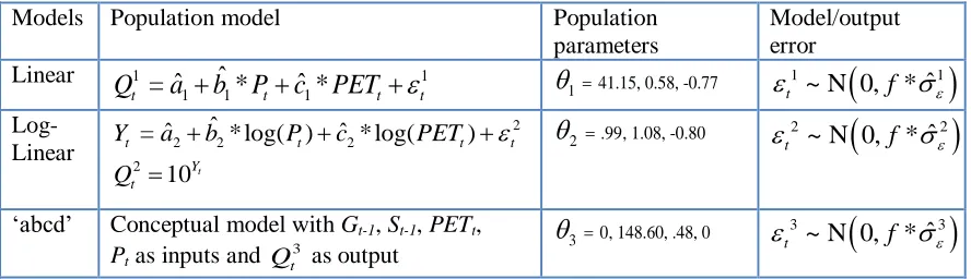
streamflow estimates perform better than the individual model estimates. Table 1 provides the structure of linear, log-linear and ‘abcd’ model. The true streamflow is generated using one of these watershed models based on the observed precipitation and potential
evapotranspiration available for the Tarboro site. We use the observed winter precipitation (Pt), streamflow (Qt) and potential evapotranspiration (PETt) for the Tar River at Tarboro to
estimate the population parameters by minimizing the sum of squares of errors between the observed streamflow and the model predicted streamflow.
Table 1: Summary of candidate stochastic streamflow generation models used in the synthetic study as well as for individual model evaluations
Models Population model Population
parameters
Model/output error
Linear 1 1
1 ˆ1 1
ˆ ˆ
= * *
t t t t
Q a b Pc PET
1 41.15, 0.58, -0.77Log-Linear
2
2 2 2
2
ˆ
ˆ ˆ
= * log( ) * log( )
10t
t t t t
Y t
Y a b P c PET
Q
2 .99, 1.08, -0.80
‘abcd’ Conceptual model with Gt-1, St-1, PETt,
Pt as inputs and Qt3 as output
3 0, 148.60, .48, 0
Using the population parameters specified in Table 1, we generate true streamflow,
j t
Q
where j denotes the hydrologic model index, from each watershed model using the observed precipitation and PET. It is important to note that the true flows also contain a model or output error ( jt
), which follows Gaussian noise with zero mean and standard deviation, f* ˆj
, where ‘f’ denotes a factor that control the residual standard deviation ( ˆj
)
for model ‘j’. The residual standard deviation ( ˆ j
) for a given model is estimated based on
1 ˆ1
~ N 0, *
t f
2 ˆ2
~ N 0, *
t f
3 ˆ3
~ N 0, *
t f
the residuals between the observed winter streamflow and the model-estimated flow. For f=0, the generated flow does not have any model error resulting in flows being exactly as that of model estimates for the Tar River at Tarboro. The model error is added explicitly to the model-estimated flow to generate many realizations of true flows. The true flows from the population models allow us to compare between single model streamflow predictions and various streamflow multimodel schemes developed using the precipitation forecasts. The next section describes the candidate single models and multimodels that are available for inter-comparison.
2.3 Single Model Forecasts Development and Evaluation Methodology
Based on the details given in Sections 2.2 and 2.3, we generate 35 years of synthetic climate forecasts based on the chosen α and β and then force it with a candidate model, j, in Table 1 to develop 35 years of synthetic streamflow forecasts. We also obtain the true streamflow, Qtj, by using the observed precipitation and PET for the 35 year period using the
population parameters given in Table 1. Figure 1 shows the evaluation methodology for a single model. The generated streamflow, Qtj, is split into two sets with the first 20 years
(t=1, 2,…nc; nc denotes the number of years of calibration)of flow being used for calibration
and the remaining 15 years (t=nc+1,nc+ 2,…n; ndenotes the number of years of
evaluation)for validation. Considering the generated streamflow as the flow available for calibration, we estimate the model parameters, ˆj, using Qtj , precipitation forecasts (Pti) and
the 20-year calibration period. The calibrated parameters, ˆj, are subsequently used with precipitation forecasts (Pti) and PETt to estimate the forecasted streamflow, QSM ti j, , by the
individual model for the validation period. It is important to note that the forecasted
streamflow by a given model, j, could vary depending on the skill of precipitation forecasts, Pti, which is determined by α and β equations (1)-(6)).
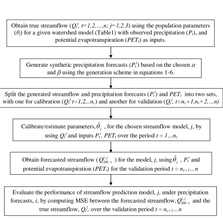
Figure 1: Flow chart for the generation of synthetic streamflow forecasts under a given climate forecasting scheme and hydrologic model
Obtain true streamflow (Qtj, t=1,2,…,n; j=1,2,3) using the population parameters
(θj) for a given watershed model (Table1) with observed precipitation (Pt), and
potential evapotranspiration (PETt) as inputs.
Generate synthetic precipitation forecasts (Pti) based on the chosen
and using the generation scheme in equations 1-6.
Calibrate/estimate parameters, ˆj , for the chosen streamflow model, j, by using Qtj and inputs Pti, PETt over the period t = 1…nc
Split the generated streamflow and precipitation forecasts (Pti) and PETt into two sets,
with one for calibration (Qtj t=1,2,..nc) and another for validation (Qtj, t=nc+1,nc+2,…n)
Obtain forecasted streamflow (QSM ti j, ) for the model, j, using ˆj , Pt
i
and potential evapotranspiration (PETt) for the validation period t = nc+1…n.
Evaluate the performance of streamflow prediction model, j, under precipitation forecasts, i, by computing MSE between the forecasted streamflow,QSM ti j, and the
We also consider a conceptual watershed model, abcd, for estimating the single model forecasts of streamflow. The ‘abcd’ model originally suggested by Thomas (1981) has been employed by various monthly and annual water balance studies (Vogel and
Sankarasubramanian, 2000; Sankarasubramanian and Vogel, 2002a). For details, see
Sankarasubramanian and Vogel (2002b). For forecasting the winter streamflow using ‘abcd’ model, apart from Pti and PETt, the model also requires initial soil moisture and groundwater
states, St-1 and Gt-1, over the calibration and validation period. We upfront develop these
estimates, St-1 and Gt-1, over the entire 35 year period by simulating the ‘abcd’ model at
seasonal time scale using observed precipitation and potential evapotranspiration and the model parameters (shown in Table 1) over the entire 35 years of record. Thus, for forecasting each year winter streamflow, we use the simulated initial soil moisture and groundwater states along with Pti and PETt for performing calibration and validation. Given the single
model streamflow forecasts, we combine them next to develop multimodel streamflow forecasts.
2.4 Multimodel Precipitation and Streamflow Forecasts Development
Models invariably contain model errors due to different sources including quality of input data, initial states of the model, parameter estimation and the inability of the model to perfectly replicate the actual physical process (Feyen et al., 2001). In recent years,
2007; Devineni et al., 2008; Devineni and Sankarasubramanian, 2010) have shown that combining different competing single models result in improved predictions. Multimodel predictions are also able to capture the strength of the single models which results in improved predictability (Ajami et al., 2007; Duan et al., 2007; Devineni et al., 2008).
When considering multimodel combination there are various methods available using weighted averages, including simple or weighted average of single model predictions
(Georgakakos et al., 2004; Shamseldin et al., 1997; Xiong et al., 2001). Other studies have explored statistical techniques such as multiple linear regression (Krishnamurthi et al., 1999) and Bayesian model averaging (Duan, et al., 2007) for multimodel combinations. In this study, multimodel combinations are obtained from single models by using weights which are obtained based on the performance of the single model over the calibration period.
For combining different synthetic precipitation/streamflow forecasts to develop multimodel forecasts, we combine models based on their ability to predict during the calibration period. Given the precipitation forecasts, i
t
P , over the calibration period (20 years), we compute the skill of the issued precipitation forecast by computing the mean square error between the forecasted mean, i
t
P , and the observed precipitation, Pt, using
equation (7). Given that we have nm climate forecasts from the synthetic scheme in Section
2.1, we obtain weights for individual models by giving higher weights for the
best-performing model (equation 8). Using the weights, Wi, obtained for each model, we obtain
multimodel precipitation forecasts,PMM t , over the validation period. One could obtain
combination (Rajagopalan et al., 2002) or optimal model combination conditioned on the predictor state (Devineni and Sankarasubramanian, 2010). Those approaches are not pursued here, since the focus is to compare the three strategies proposed in the introduction.
Application of such methods will only result in further improvements in multimodel predictions.
2
1
( ) ...(7)
c
n
i
i t t
t
MSE P P
1 1 1 ...(8) m i i n i i MSE W MSE
1* 1, 2, ..., ...(9)
m
n i
MM t t i c c
i
P P W t n n n
Similar to multimodel combination on precipitation forecasts, we also combine the streamflow forecasts, ,
( 1, 2..., ; 1, 2,3)
i j
SM t m
Q i n j , developed from individual models with different synthetic precipitation forecasts. To begin with, we first compute mean square error between the single model prediction, i j,
SM t
Q and the true flow for the model, Qtj, over the
calibration period (t=1,2,..nc). This results in a total of nm*3 MSE estimates from different
(12) over the validation period. This basically gives the multimodel forecasts corresponding to the second strategy MM-Q.
, 2 ,
1
( ) ...(10)
c
n
j i j
i j t SM t
t
MSE Q Q
1 , , 1 , , ...(11) i j i j i j i j MSE W MSE
, , ,* 1, 2, ..., ...(12)
i j
MM Q t SM t i j c c
i j
Q Q W t n n n
2.5 Streamflow Predictions – Candidate Single Models and Multimodels To evaluate the three strategies proposed in the introduction for reducing the
uncertainty in streamflow predictions, we also need candidate streamflow prediction models that estimate the streamflow forecasts for the given precipitation forecasts. Synthetic
precipitation forecasts with different skills could be generated using equations (1) - (6) for the 35-year period with each year forecast being represented with 100 realizations. The ensemble mean is used as the forecast inputs for the streamflow prediction models. The first model is the single model setup in which the individual synthetic precipitation forecasts ( i
t
P )
is be used with one of the streamflow prediction models (Table 1) to obtain the modeled streamflow ( i j,
SM t
Q ). Thus, in the individual model streamflow predictions denoted as i j,
SM t
Q
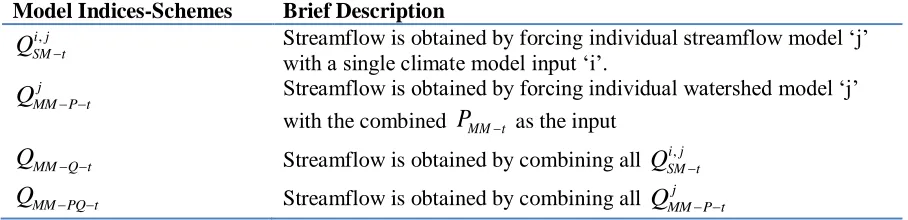
Table 2: Summary of streamflow forecasts developed from different climate and hydrology model combinations
Model Indices-Schemes Brief Description
,
i j SM t
Q Streamflow is obtained by forcing individual streamflow model ‘j’ with a single climate model input ‘i’.
j MM P t
Q Streamflow is obtained by forcing individual watershed model ‘j’ with the combined PMM t as the input
MM Q t
Q Streamflow is obtained by combining all QSM ti j,
MM PQ t
Q Streamflow is obtained by combining all QMM P tj
The first strategy, MM-P, reduces the input uncertainty first by combining the synthetic precipitation forecasts to develop multimodel precipitation forecasts,PMM t , which
are then used as an input with the streamflow prediction model (Table 1), j, to obtain streamflow ( j
MM P t
Q ). Details and steps involved in multimodel combination of precipitation
and streamflow are given in the previous section. The second strategy, MM-Q, reduces the uncertainty in streamflow prediction by first ingesting the individual synthetic climate forecasts (without multimodel combination) with the individual watershed models and then combines the individual streamflow ( i j,
SM t
Q ) to obtain a multimodel streamflow which is denoted by QMM Q t . Thus, the strategy, MM-P, uses multimodel precipitation forecasts to obtain streamflow, while the MM-Q method combines the streamflow forecasts obtained from various individual models. The third strategy, MM-PQ, combines all j
MM P t
Q obtained from the strategy MM-P to obtain QMM PQ t . The multimodel modeled streamflow, QMM P tj
In summary, we have streamflow predictions from single models, i j,
SM
Q and three multimodel combinations j
MM P
Q , QMM Q and QMM PQ as shown in Table 2. The performance
of these streamflow predictions is evaluated using mean square error, which is computed based on the streamflow predictions and the true model streamflow Qtj during the validation
period t = nc+1…n. For each climate model precipitation i and model index j, the evaluation
of streamflow predictions i j,
SM
Q gives a single value of mean square error. The first multimodel combination, MM-P, denoted by j
MM P
Q yields a single value of mean square error for each model index, j. The second and third multimodel combinations denoted by
MM Q
CHAPTER 3 Results
In this chapter, we compare the performance of single models and the three
multimodel strategies based on the estimated mean square error from 1000 realizations. The first section presents results from three precipitation forecasts forced with the linear
streamflow prediction model (Table 1). The true flows, 1
t
Q , are also generated from the linear model. Given that we have only one streamflow prediction model, the third strategy, MM-PQ, is non-existent resulting in comparison between MM-P and MM-Q. The primary question that we address under this analysis is: Given no hydrologic model uncertainty, what is the best way to reduce uncertainty in streamflow forecasts using precipitation forecasts available from multiple models?
In the second section, we consider three streamflow prediction models (Table 1) with the true streamflow being generated from one of the hydrologic model. Thus, under this case, we explicitly consider uncertainties across climate models and hydrologic models by
analyzing the proposed three strategies, MM-P, MM-Q and MM-PQ, for reducing the uncertainty in streamflow forecasts based on MSEs from 1000 realizations. This helps us to pick the right strategy that will reduce uncertainty in streamflow predictions by considering both input (precipitation) uncertainty and output (streamflow) uncertainty.
3.1 Streamflow Predictions – Candidate Single Models and Multimodels
precipitation forecasts with different skills by varying α and β. Each precipitation forecast is used with the candidate model – linear streamflow prediction model – to estimate three single model streamflows denoted by i
SM
Q . The first multimodel combination streamflow, QMM P ,
is derived by combining the three precipitation forecasts and then the combined precipitation forecasts, PMM, is used with the linear model. The second multimodel combination
streamflow, QMM Q , is derived by combining the streamflow from the single models ( i SM
Q ;
i=1,2,3). We basically repeat the procedure in Figure 1 1000 times to develop 1000 estimates
of MSEs. Similarly, we also obtain MSEs, QMM P and QMM Q , by repeating the procedure in Section 2.4.
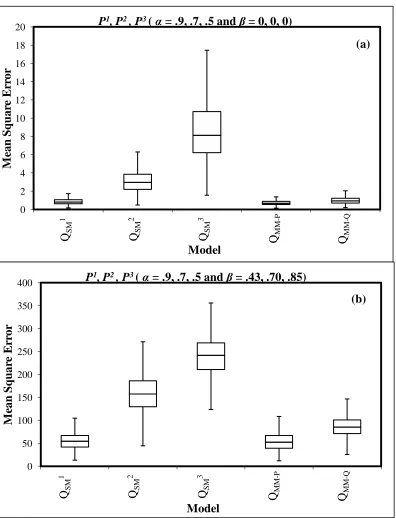
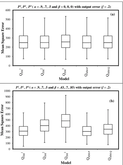
To begin with (Figure 2), we consider precipitation forecasts with varying skills by adjusting values for α and also by allowing the forecasts to be well-dispersed (Figure 2a) or overconfident (Figure 2b) based on β. It is important to note that in evaluating the
precipitation forecasting schemes, we compare their ability to predict the true streamflow arising from the same population model. It is obvious from Figure 2a, skillful forecasts have lesser MSEs compared to the streamflow estimated by using lower skillful forecasts.
Figure 2: Box-plots of MSEs in predicting streamflow estimated by a linear model for (a) well-dispersed (β = 0) precipitation forecasts having different correlations (α = .9, .7, .5) and (b) over-dispersed (β ≠0) precipitation forecasts having different correlations (α = .9, .7, .5)
0 2 4 6 8 10 12 14 16 18 20 M ean S q u ar e E rr or Model
P1, P2 , P3( α = .9, .7, .5 and β = 0, 0, 0)
QSM 1 QSM 2 QSM 3 QMM -P QMM -Q 0 50 100 150 200 250 300 350 400 M ean S q u ar e E rr or Model
P1, P2 , P3 ( α = .9, .7, .5 and β = .43, .70, .85)
Figure 3: Box-plots of MSEs in predicting streamflow estimated by a linear model with the true streamflow generated with output error (f=0.2) for (a) well-dispersed (β = 0)
precipitation forecasts having different correlations (α = .9, .7, .5) and (b) over-dispersed (β ≠0) precipitation forecasts having different correlations (α = .9, .7, .5)
0 100 200 300 400 500 600 M ean S q u ar e E rr or Model
P1, P2 , P3 ( α = .9, .7, .5 and β = 0, 0, 0) with output error (f = .2)
QSM 1 QSM 2 QSM 3 QMM -P QMM -Q (a) 0 100 200 300 400 500 600 700 800 900 1000 M ean S q u ar e E rr or Model
P1, P2 , P3 ( α = .9, .7, .5 and β = .43, .7, .85) with output error (f = .2)
The single models perform better as the skill of the precipitation increases. We also see that the two multimodels (MM-P and MM-Q) perform better due to reduction in climate model uncertainty. Both multimodel combinations improve performance by reducing uncertainty. It is important to note that MM-P performs very close to the best-performing individual model. Since the skill of the precipitation forecast is not the same
(varying values for α), we have used varying weights to combine the precipitation and streamflow used in the multimodels. Due to the varying weights we can observe that the multimodel combinations can perform better than the best single model (model with the highest value of α) as shown in Figure 2(a). The multimodel combination QMM P (reducing
input uncertainty) performs better than the best single model and the QMM Q (reducing output uncertainty) multimodel. This implies that for systematic uncertainty reduction in
streamflow, we need to reduce input (precipitation) uncertainty first, so that the estimated streamflow using multimodel climate forecast performs better than streamflow forecasts derived without any reduction in input uncertainty. This is mainly because reduced
uncertainty in the inputs to the watershed model results in better accuracy in predicting the true streamflow arising from the same model. So regardless of the whether the precipitation forecast is well-dispersed or overconfident, the improvement in performance is better if one reduces the input uncertainty rather than the output uncertainty. Furthermore, both
In Figure 2, we did not consider the hydrologic model error or output error by forcing the term f=0 in synthetic streamflow generation. By selecting f=0.2, Figure 3 shows the performance of different models under a well-dispersed and over-confident precipitation forecasts with varying β. Figure 3a shows that the performance of the multimodel, MM-P, is just as good as the best-performing streamflow prediction scheme forced with a highly skillful well-dispersed precipitation forecast. From Figure 3b, we see that as the forecasts become overconfident, MM-P performs better than MM-Q as well as the best-performing single model predictions. These findings are completely in line with Weigel et al. (2008) who showed that multimodel combinations result in better predictions as the model dispersion increases. In the case of well-dispersed forecasts, the performance of multimodel predictions is just as good as the best-performing individual model predictions.
3.2 Source of Model Uncertainty - Climate Models and Hydrologic Models
In the previous section we considered only the linear model to be the candidate and the population hydrologic model. In this section we consider all three models (in Table 1) to be candidate models with the true streamflow being generated by either linear model or ‘abcd’ watershed model. Similar to the previous section, we consider three precipitation forecasts having different skills. Each precipitation forecast is forced with the three streamflow prediction models to develop nine streamflow forecasts, i j,
SM
multimodel combination streamflows ( j MM P
Q with j = 1,2,3). The streamflow from nine single models i j,
SM
Q is combined using equations (10)-(12) to develop multimodelQMM Q . Similarly, streamflow forecasts from three multimodel j
MM P
Q is combined separately (using equations (10)-(12)) to develop multimodel streamflow forecasts, QMM PQ , which reduces first the input uncertainty followed by output uncertainty. Thus, in this section, we present MSEs from 14 models that include nine single models and five multimodels. All the
multimodel combinations on precipitation/ streamflow are obtained using weights dependent upon the skill of the forecast during the calibration period.
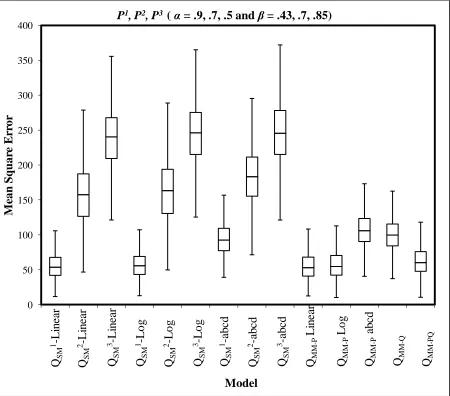
Figure 4 presents the box-plots of MSEs for 14 models with the linear model as the population model having no output error (f=0). From Figure 4, we can see that the abcd
SM
Q and
abcd MM P
Q perform the worst across all the models. This is partly because the assumed watershed model is linear and the ‘abcd’ model is a nonlinear water balance model. The multimodel combinations, QMM P , that reduces first the input uncertainty performs better than their
counterpart forced with individual model precipitation forecasts. We can see that in the case of the linear candidate model, Linear
MM P
Q performs better than the best single model Q1,SMLinear.
than the multimodel combination QMM PQ . This is to be expected since QMM PQ reduces
input and output uncertainty by combining the streamflow from the multi-modes combination QMM P rather than the single models.
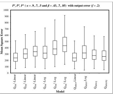
Figure 4: Box-plots of MSEs for 1000 realization for three candidate streamflow prediction models with the true streamflow arising from linear model (f=0) and the precipitation forecasts having different skill (α = .9, .7, .5) and dispersiveness (β = .43, .7, .85)
0 50 100 150 200 250 300 350 400 M ean S q u ar e E rr or Model
P1, P2, P3 ( α = .9, .7, .5 and β = .43, .7, .85)
Figure 5: Same as Figure (4) but with streamflow output error (f =.2)
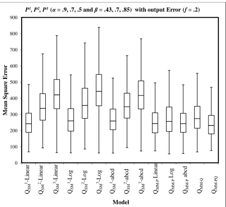
The mean square error of all models has increased in Figure 5 primarily due to the noise added to the true model streamflow (f = .2). But the relative performance of the single and multimodel combinations has remained the same. Forcing the candidate watershed model with multimodel precipitation forecasts, MM-P, improves the performance of three candidate models. Similarly, streamflow forecasts developed based on the strategy, MM-PQ,
0 100 200 300 400 500 600 700 800 900 M ean S q u ar e E rr or Model
P1, P2, P3 (α = .9, .7, .5 and β = .43, .7, .85) with output Error (f = .2)
perform better than MM-P and MM-Q when output error is present. Thus, to reduce the uncertainty in streamflow prediction, it is important to first reduce the input uncertainty, which needs to be followed with reduction in hydrologic model uncertainty.
Figure 6: Same as Figure 5, but the true flows arise from ‘abcd’ model with output error (f =.2) 0 100 200 300 400 500 600 700 800 900 1000 M ean S q u ar e E rr or Model
P1, P2, P3( α = .9, .7, .5 and β = .43, .7, .85) with output Error (f = .2)
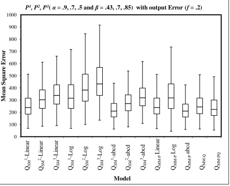
Figure 7: Same as Figure 6, but without ‘abcd’ model among the candidate models
In all previous results we have considered the true streamflow generation model along with the candidate model available for developing streamflow forecasts. We also considered how various candidate single models and multimodels perform when the true streamflow arises from a population model that is not part of the candidate models. In Figure 7, we perform the same analysis by excluding ‘abcd’ model from the candidate model. Thus, we consider the linear and log-linear to be the candidate models. Thus, we have a total of six
0 100 200 300 400 500 600 700 800 900 1000 M ean S q u ar e E rr or Model
P1, P2, P3 ( α = .9, .7, .5 and β = .43, .7, .85) with output error (f = .2)
single model forecasts ( i j,
SM
Q ), two single model predictions forced with multimodel precipitation forecast ( j
MM P
Q ), one multimodel predictions (QMM Q ) from
,
i j SM
Q and one multimodel predictions (QMM PQ ) based on QMM Pj . This results in a total of 10 prediction
schemes available for evaluation. Based on Figure 7, the best-performing models are Linear MM P
Q
and QMM PQ . Though the median of QMM PQ is slightly higher than that of Linear MM P
Q , the difference in the MSE between the two schemes is very marginal.
In this chapter we have considered reducing only climate model uncertainty and both climate and hydrological model uncertainty as a means of reducing uncertainty in the
streamflow predictions by analyzing three proposed strategies, MM-P, MM-Q and MM-PQ. When considering no hydrological model uncertainty, reducing input uncertainty by using MM-P strategy performs better than reducing output by using MM-Q regardless of whether the precipitation forecasts is well-dispersed or overconfident. We can attribute this to the fact that reduced uncertainty in the inputs of the watershed model results in better accuracy in predicting the true streamflow arising from the same model. While we only consider the linear model to be the population and candidate model in Section 3.1, the same conclusions can be reached if one uses other model, log or ‘abcd’ model, for either population or
CHAPTER 4 Application
The results discussed so far have been based on a synthetic model. In this section, we investigate how the proposed multimodel combination strategies perform in predicting the observed streamflow at Tar River at Tarboro (Figure 8). The observed winter seasonal streamflow and potential evapotranspiration are obtained for the Tar River at Tarboro site (02083500) from the HCDN database of Vogel and Sankarasubramanian (2005). The
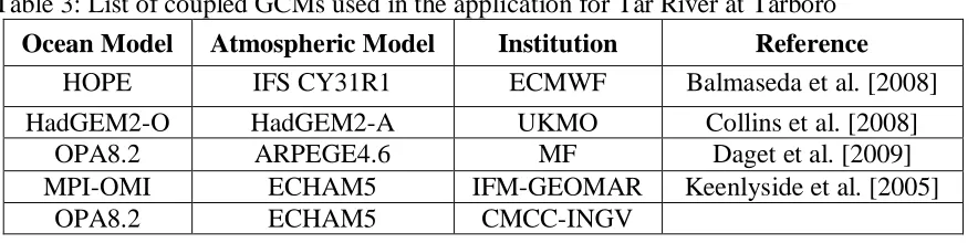
precipitation forecasts for Tar River at Tarboro are obtained from five coupled GCMs (Table 3) developed as part of the ENSEMBLES project (Devineni, N., and A. Sankarasubramanian 2010). The precipitation forecasts from eight grid points over the domain (longitude -80W to 75W; latitude-32.5N to 37.5N) available at a monthly time step from 1981 to 1999 are considered for developing winter streamflow forecasts. The monthly precipitation forecasts issued in November from each GCM are converted into seasonal precipitation forecasts over the period January-March for further analysis.
Table 3: List of coupled GCMs used in the application for Tar River at Tarboro Ocean Model Atmospheric Model Institution Reference
HOPE IFS CY31R1 ECMWF Balmaseda et al. [2008]
HadGEM2-O HadGEM2-A UKMO Collins et al. [2008]
OPA8.2 ARPEGE4.6 MF Daget et al. [2009]
MPI-OMI ECHAM5 IFM-GEOMAR Keenlyside et al. [2005]
Figure 8: Location of the Tar River at Tarboro along with the latitude and longitude of the eight grid points used for the analysis
The precipitation from the five GCMs (Table 3) (i = 1…5) is used with the candidate models (j = 1…3) to obtain the single model streamflow i j,
SM
Q . There are fifteen single models which are combined to obtain the multimodel streamflow denoted by QMM Q . The multimodel precipitation data is based on the algorithm developed by Devineni and
Sankarasubramanian (2010) which considers the forecasted Nino3.4 from each GCM as the
conditioning variable. The multimodel streamflow j MM P
Q is obtained by using the multimodel precipitation with the candidate model j. The final multimodel combination
MM PQ
Q is obtained by combining the three QMM Pj streamflow. The winter precipitation
of each GCM is spatially correlated, we can use Principal Component Analysis to obtain a single time series which explains the maximum variance of the original eight grids of the GCM. Generally the downscaled precipitation has better correlation than the eight grid points.
Figure 9: Mean square error of individual GCMs and multimodel combination schemes in predicting the observed streamflow for the Tar River at Tarboro. The analysis considers three hydrological models linear, log-linear and ‘abcd’ model
6441 7225 6160 8453 8525 5850 6739 7005 5902
8602 8614
6518 9673
8137
10153 10219 10289
6957 7520 5772 5000 6000 7000 8000 9000 10000 11000 QSM -C MC C QSM -E C MW F QSM -F R A N C E QSM -G EO MA R QSM -UK MO Q MM -P Q MM -Q Q MM -PQ M ean S q u ar e E rr or
Figure 10: Multimodel streamflows plotted with the observed streamflow at Tar River
In order to evaluate the performance of the various multimodel methods, we use a calibration and validation approach as described in the experimental design section with mean square error as the performance metric. The first 20 years of data (1961-1980) are used to calibrate the various hydrological models while the last 19 years (1981-1999) are used for validation. The models are calibrated and validated using the observed streamflow, potential evapotranspiration and precipitation data from the five single GCMs and multimodel
algorithm. The results from the application are presented in Figure 9 during the validation period (1981-1999).
0.00 20.00 40.00 60.00 80.00 100.00 120.00 140.00
0 2 4 6 8 10 12 14 16 18 20
S
tr
eam
fl
ow
(m
m
/m
on
th
)
Validation Years
Observed vs Multimodel Streamflow for Tar River
QMM-Q Q
Multimodel and observed streamflow are plotted in Figure 10. The results obtained in this analysis verify the results obtained through the synthetic model setup. It is clear that employing multimodel combination improves performance over single models. We also see that reducing the input uncertainty (climate models) through multimodel combinations is more critical than reducing output uncertainty (hydrological models) (the results for MM-Q for each candidate model are not shown in Figure 9). The overall best performance is
CHAPTER 5 Conclusions
Given that we have climate forecasts from multiple climate models, which could be ingested with multiple watershed models, a systematic analysis is performed for identifying the right strategy to reduce the uncertainty in streamflow forecasts. The methodology considers reducing the input uncertainty first by combining climate forecasts and then uses those multimodel climate forecasts as inputs with multiple watershed models. We further combined the streamflow predictions obtained using multimodel climate forecasts to develop a forecast that reduces uncertainties in climate models and hydrologic models. We also considered combining streamflow predictions developed by forcing individual climate models with individual watershed models. Considering the synthetic precipitation forecast scheme suggested by Weigel et al. to generate climate forecast, the study considers three streamflow prediction models linear, log-linear and ‘abcd’ model as candidate models. Based on the synthetic models and application for Tar River, we reach the following conclusions: (a) Multimodel streamflow obtained either by reducing input (climate forecast) or output
(hydrologic model) uncertainty performs better than the streamflow predictions obtained from single models even if we employ the single models having the true model form. (b) Reducing the input (climate forecast) uncertainty through multimodel combinations is
more critical than reducing output (hydrologic model) uncertainty.
(d) When considering multiple candidate models, reducing input (climate forecast) uncertainty followed by reducing output (hydrologic model) uncertainty will provide better results than only reducing output (hydrologic model) uncertainty.
REFERENCES
Ajami, N. K., Q. Duan, and S. Sorooshian (2007), An integrated hydrologic Bayesian multimodel combination framework: Confronting input, parameter, and model structural uncertainty in hydrologic prediction, Water Resour. Res., 43, W01403,
doi:10.1029/2005WR004745.
Barnston AG, Mason SJ, Goddard L, DeWitt DG, Zebiak SE. 2003. Multimodel ensembling in seasonal climate forecasting at IRI. Bulletin of the American Meteorological Society, 1783–1796, DOI:10.1175/BAMS-84-12-1783.
Chowdhury, S., and A. Sharma, 2009: Long-range Nin˜ o-3.4 predictions using pairwise dynamic combinations of multiple models. J. Climate, 22, 793–805.
Devineni, N., and A. Sankarasubramanian 2010, "Improved Categorical Winter Precipitation Forecasts Through Multimodel Combinations of Coupled GCMs." GEOPHYSICAL
RESEARCH LETTERS 37(2010): . Print.
Duan, Q., N. K. Ajami, X. Gao, and S. Sorooshian (2007), Multi-model ensemble hydrologic prediction using Bayesian model averaging, Adv. Water Resour., 30(5), 1371–1386,
doi:10.1016/j.advwatres.2006.11.014.
Georgakakos, K. P., D.-J. Seo, H. V. Gupta, J. Schaake, and M. B. Butts (2004),
Characterising streamflow simulation uncertainty through multimodel ensembles. J. Hydrol., 298(1–4), 222–241.
Goddard, L., A. G. Barnston, and S. J. Mason, 2003: Evaluation of the IRI’s ‘‘net
assessment’’ seasonal climate forecasts: 1997–2001. Bull. Amer. Meteor. Soc., 84, 1761– 1781.
Krishnamurti, T. N., C. M. Kishtawal, T. E. Larow, D. R. Bachiochi, Z. Zhang, C. E. Williford, S. Gadgil, and S. Surendran (1999), Improved weather and seasonal climate forecasts from multimodel superensemble. Science, 285, 1548–1550.
Luo, L. and E. F. Wood (2008), Use of Bayesian merging techniques in a multi-model seasonal hydrologic ensemble prediction system for the Eastern U.S. J. Hydrometeo.,5, 866-884
Mahanama, S. P. P., B. Livneh, R. D. Koster, D. Lettenmaier, and R. H. Reichle, 2012: Soil moisture, snow, and seasonal streamflow forecasts in the United States. J. Hydrometeor., in press.
Marshall, L., D. Nott, and A. Sharma (2005), Hydrological model selection: A Bayesian alternative, Water Resour. Res., 41, W10422, doi:10.1029/2004WR003719.
Marshall, L., A. Sharma, and D. Nott. 2006. Modeling the catchment via mixtures: Issues of model specification and validation. Water Resources Research 42(11):1-14.
Marshall, L., A. Sharma, D. Nott. 2007. A single model ensemble versus a dynamic
modeling platform: Semi-distributed rainfall runoff modeling in a Hierarchical Mixtures of Experts framework. Geophysical Research Letters, 34, L01404,
Marshall, L., A. Sharma, and D. Nott. 2007. Towards dynamic catchment modelling: a Bayesian hierarchical mixtures of experts framework. Hydrological Processes 21(7), 847-861, DOI: 10.1002/hyp.6294.
Overgaard, J., D. Rosbjerg, and M. B. Butts (2006), Land-surface modeling in hydrological perspective––A review, Biogeosci., 3, 229–241.
Oudin, L., Perrin, C., Mathevet, T., Andréassian, V. and Michel, C., 2006. Impact of biased and randomly corrupted inputs on the efficiency and the parameters of watershed models. Journal of Hydrology 320, 62-83, doi:10.1016/j.jhydrol.2005.07.016.
Rajagopalan, B., U. Lall, and S. E. Zebiak (2002), Categorical climate forecasts through regularization and optimal combination of multiple GCM ensembles. Mon. Wea. Rev., 130, 1792–1811.
Regonda, S. K., B. Rajagopalan, M. Clark, and J. Pitlick (2005), Seasonal cycle shifts in hydroclimatology over the western United States, J. Clim., 18, 372–384.
Sankarasubramanian, A., U. Lall, and S. Espuneva, 2008: Role of retrospective forecasts of GCM forced with persisted SST anomalies in operational streamflow forecasts development. J. Hydrometeor., 9, 212–227.
Shamseldin, A. Y, K. M. O’Connor, and G. C. Liang (1997), Methods for combining the outputs of different rainfall-runoff model, J. Hydrol., 197, 203– 229.
Sinha and Sankarasubramanian, 2012, Role of Climate Forecasts and Initial Land-Surface Conditions in Developing Operational Streamflow and Soil Moisture Forecasts in a Rainfall-Runoff Regime: Skill Assessment, Hydrology and Earth System Sciences, Under Review.
Thomas, H. A., Improved methods for national water assessment, report contract WR 15249270, U.S. Water Resour. Counc., Washington, D. C., 1981.
Vogel, R. M., and A.Sankarasubramanian (2005), USGS Hydro-Climatic Data Network. (HCDN): Monthly Climate Database, 1951-1990.
Vogel,R.M. and A.Sankarasubramanian,Scaling Properties of Annual Streamflow in the continental United States,Journal of Hydrological Sciences,45,465-476,2000.
Vrugt, J.A., O´ Nualla´in, B., Robinson, B.A., Bouten, W., Dekker, S.C., Sloot, P.M.A., 2006. Application of parallel computing to stochastic parameter estimation in environmental models. Computers and Geosciences 32 (8), 1139–1155. doi:10.1016/ j.cageo.2005.10.015.
Vrugt, J. A., and B. A. Robinson (2007), Treatment of uncertainty using ensemble methods: Comparison of sequential data assimilation and Bayesian model averaging, Water Resour. Res., 43, W01411, doi:10.1029/2005WR004838.
Wood, A. W., Maurer, E. P., Kumar, A., and Lettenmaier, D. P.: Long-range experimental hydrologic forecasting for the Eastern United States, J. Geophys. Res., 107, 4429,
doi:10.1029/2001JD000659, 2002.
Xiong, L. H., A. Y. Shamseldin, and K. M., O’Connor (2001), A nonlinear combination of the forecasts of rainfall-runoff models by the first order Takagi-Sugeno fuzzy system. J. Hydrol. 245 (1–4), 196–217.
Xu, C.Y. and Singh, V.P. (2004) Review on Regional Water Resources Assessment Models under Stationary and Changing Climate. Water Resour. Manag., 18, 591–612.