Transactions, SMiRT-25 Charlotte, NC, USA, August 4-9, 2019
Division III - Computation, Simulation, Visualization
STUDYING THE EFFICIENCY OF ANTI-EXPLOSION PROTECTIVE
STRUCTURES USING ADVANCED NUMERICAL SIMULATION
Charisis T. Chatzigogos1, Yannick Chaveau2, Pierre-Alain Nazé3
1 R&D Group, Géodynamique & Structure, Paris, France ([email protected]) 2 Rapid Dynamics Group Leader, Géodynamique & Structure, Paris, France
3 CEO, Géodynamique & Structure, Paris, France
ABSTRACT
This paper presents a concise methodology for studying the efficiency of protective structures encountered in open circuits of nuclear facilities using advanced numerical simulation. The scope of such protective structures is to attenuate the intensity of pressure waves that originate from external explosions or extreme climatic phenomena (such as tornados). The performance assessment for such structures requires to model: a) the propagation domain upstream of the structure b) the domain of the structure itself, with all relevant structural and geometric details and c) the propagation domain downstream of the structure. Crucial steps in setting up an efficient numerical model for such problems are: the selection of an appropriate method for the consideration of fluid-structure interaction, the selection of a time integration scheme for modelling the pressure wave propagation and the construction of an adapted finite element mesh for the three studied domains. The paper presents an application of the proposed method for assessing the performance of a typical protective structure and comments on the type of results that can be obtained with this approach.
INTRODUCTION
This paper presents a complete modelling procedure for studying the efficiency of protective structures encountered in open circuits of large industrial and nuclear facilities using advanced numerical simulation. The scope of such protective structures is to attenuate the intensity of pressure waves or wind action that originate from external explosions or extreme climatic phenomena (such as tornados) and are susceptible of attaining critical zones or equipment, through an open circuit (e.g. ventilation circuit) of an industrial facility. The protective structures typically consist of a steel frame and a grid of steel elements (thin plates and/or hollow tubes) that serve for the attenuation of the incident pressure waves via multiple reflections and refractions. The performance criteria desired for these structures are: a) to be able to withstand structurally the incident actions, b) to lead to an attenuation of the actions (downstream) up to a prescribed performance level and c) to respect some lighting or ventilation criteria related to the circuit, in which they are installed.
The performance assessment for such protective structures leads to non-trivial problems of pressure wave propagation and fluid-structure interaction, in which it is necessary to model: a) the propagation domain upstream of the structure, to allow for a rigorous modelling of the incident and the reflected pressure waves, b) the domain of the structure itself, with all relevant structural and geometric details and c) the propagation domain downstream of the structure, to assess the performance of the protective structure in attenuating the incident wave. Crucial steps in setting up an efficient numerical model for such problems are:
I. The selection of an appropriate method for the consideration of fluid-structure interaction:
The structure displacements are thus practically negligible with respect to fluid flow; this allows modelling the structure as an infinitely rigid obstacle which does not interact with the fluid domain (for which, an eulerian formulation can be adopted). If it is shown that the structure displacements are significant (nonlinear structural response), a more suitable formulation must be adopted for the propagation domain (e.g. ALE: Arbitrary Lagrange-Euler), in conjunction with the structure domain, to model rigorously the incumbent fluid-structure interactions.
II. The selection of an appropriate time integration scheme for the problem of pressure wave
propagation: the time scales relevant to explosion problems (~1s) typically lead to the use of an explicit (conditionally stable) time integration scheme.
III. Finally, the construction of an appropriate global finite element mesh for the three relevant domains (upstream / structure / downstream). The properties of the finite element mesh strongly influence the definition of the critical time step of the explicit scheme and the overall efficiency of the model, so an elaborate mesh optimization procedure is followed in order to satisfy the best possible compromise between accuracy and calculation speed.
Géodynamique & Structure (GDS), a major design consultancy in the French Nuclear Industry, exhibits strong expertise on the study of nuclear facilities under severe accidental actions. In particular, GDS has conducted several studies and R&D activities in developing methods for assessing the efficiency of anti-explosion protective structures. The scope of the present paper is to present a state-of-the-art methodology for performing this task via a real application. Emphasis is given on the modelling subtleties of the proposed approach and on the versatility of the obtained results.
BASIC ASSUMPTIONS FOR THE STUDY
The anti-explosion protective structures under study are three-dimensional steel grids placed within circuits or openings in structural elements, with the objective of attenuating incident pressure waves or wind action, while respecting some lighting or ventilation criteria. The dimensions of the grids may vary according to the dimensions of the opening/circuit to be protected (typically around 500mm to 1000mm). The essential feature of these grids is that they are constituted of steel elements, oriented along the three spatial dimensions and forming an internal skeleton whose role is to achieve the attenuation of the incident wave by means of multiple reflections and refractions. The steel elements are typically bent steel plates with a given thickness (lamellas) or steel cylinders; these elements are placed parallel and/or perpendicularly to one another. It is possible to define the “opacity” 𝑜 of the protective structure which is the ratio of the volume occupied by the steel elements 𝑉 over the total volume 𝑉 of the opening to be protected: 𝑜 = 𝑉 /𝑉 . The efficiency of the structure is thus to provide the biggest possible attenuation of the incident action for a given opacity. This is a problem of structural optimization and its solution depends on the shape of the opening to be protected and the type of incident action. In the following, we will consider a generic protective grid without entering into the discussion of the optimal disposition of the lamellas and cylinders. We will rather concentrate on the methodology for studying the efficiency of such a protective grid in attenuating a typical explosion-generated pressure wave.
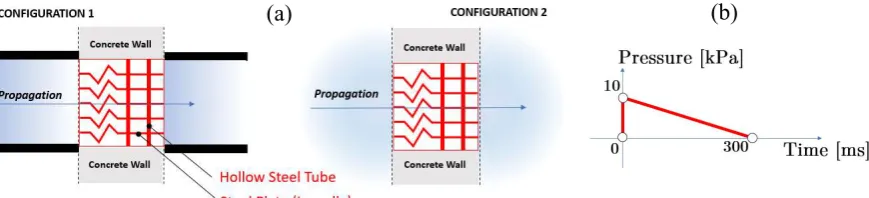
Studied configurations
Figure 1: a) Configurations of the studied protective grid, b) Definition of incident pressure wave
Definition of incident pressure wave
The incident pressure wave in the study corresponds to a triangular pulse, attaining almost instantaneously a peak pressure value of 10kPa and exhibiting a post-peak duration of 300ms. This is a typical explosion-generated pressure wave, in which the source of explosion is relatively distant with respect to the protective grid. The peak is expressed in terms of relative pressure with respect to the atmospheric pressure, implying a peak absolute pressure equal to 110kPa = 1.1bar.
Material properties
Since the grid and the concrete wall can be considered perfectly rigid, the studied problem requires the definition of a unique material which characterizes the fluid domain, which is the domain where the wave propagation takes place. The fluid, which is atmospheric air, is modelled as a perfect gas respecting the following equations:
- The ideal gas state law: 𝑃 = (1)
- Laplace’s law: 𝑃𝑉 = constant (2)
For equations (1) and (2), the following physical quantities are defined (units in brackets): - 𝑃: pressure of the ideal gas [Pa]
- 𝜌: mass density of the ideal gas [kg/m3]
- 𝑅: the universal gas constant (𝑅 = 8.314462 JK-1mol-1)
- 𝑀: the molar mass of the gas (𝑀 = 29gr/mol for atmospheric air) - 𝑇: the absolute gas temperature [K]
- 𝑉: the volume occupied by the gas [m3]
- 𝛾 = 𝐶 /𝐶 : thermal capacities ratio - 𝐶 : constant pressure thermal capacity [J/K] - 𝐶 : constant volume thermal capacity [J/K]
The mechanical parameters required for the definition of the constitutive law of the atmospheric air, modeled as perfect gas, are provided in the following Table 1. These correspond to typical values for an ambient temperature 𝑇 = 20°C.
Table 1: Mechanical parameters for atmospheric air
Mass density of atmospheric air 𝝆 [kg/m3] 1.204 Propagation velocity of sound 𝑐 [m/s] 343.21
Thermal capacities 𝛾 [-] 1.40
METHODOLOGY OF CALCULATIONS
The proposed methodology for modeling the propagation of the prescribed pressure wave entails the following steps:
a. Development of a 3D finite element mesh, representing the fluid volume contained within the grid and also in the upstream and downstream domains. The mesh is composed of 8-noded hexahedral elements, exhibiting a form as regular as possible and also a sufficient fineness for the modeling of the studied phenomena. The dimensions of the mesh in the upstream domain are defined so as to correctly reproduce the incident wave on the grid. The dimensions of the downstream domain are defined in view of quantifying the attenuation of the pressure wave up to a given distance.
b. Adoption of an appropriate formulation for solving the wave propagation problem of the pressure wave through the grid. Under the assumption of a rigid grid, an eulerian formulation is adopted for the fluid domain. The grid is modelled by constraining the nodes laying in the middle fiber of the lamellas; the exact thickness of the lamellas is modeled indirectly through an appropriate mesh discretization of the fluid domain.
c. The calculation is performed assuming “no slip” conditions in the interfaces between the fluid and the grid components. This assumption implies that there can be no relative movement (slip) of the air in contact with the grid. This assumption is concretized by constraining the three degrees-of-freedom of the nodes representing the grid structural components. The air propagates through the grid assuming conditions of laminar, compressible, Navier-Stokes flow.
d. The numerical problem is resolved using the explicit dynamics software RADIOSS, which is available in the general platform HyperWorks © by Altair (2017). The wave propagation problem is solved by direct time integration using an explicit time integration scheme. The choice for an explicit scheme is dictated by the time scale of the studied phenomena, which is of the order of ~1s, at most. The integration scheme is conditionally stable and the critical time step depends (among other things) on the smallest element size in the finite element mesh.
e. The above point (d) sets a strict requirement for a finite element mesh as regular as possible. The fineness, regularity and dimensions of the mesh are subjected to detailed validations launching the full transient dynamic analyses.
DEVELOPMENT OF FINITE ELEMENT MESH
As stated above, the assumption of a rigid grid allows modelling exclusively the fluid, which can thus be split in three domains: a) the upstream domain, b) the grid domain and c) the downstream domain. The development of a mesh for these three domains can be done independently. Once the three meshes have been developed and optimized, they can be assembled in one unique mesh for the entire fluid domain.
Grid domain
The governing geometric quantities are: a) the thickness of the lamellas 𝑡 and b) the distance ℎ between the middle fibers of two adjacent lamellas. The finite element mesh must be as regular as possible, so the elements within the grid domain should have a uniform dimension 𝑒. Given that the nodes at the middle fibers of the lamellas are constrained, this implies that their zone of influence should be equal to the mid-thickness of the lamellas, so that the mesh can reproduce correctly the thickness of the lamellas. This then yields a simple rule for determining the optimal dimension 𝑒 of volume elements, which is 𝑒 ≈ 𝑡. With this modelling option, the number of elements for discretizing the region between two lamellas is 𝑛 = ℎ/𝑡 (for mesh discretization, we can take the closest integer of this ratio). If we define as effective section of the mesh, the zone of influence of the nodes with free degrees-of-freedom (cf. Figure 2a), the above modeling option leads to an effective section, which is equal to ℎ = (𝑛 − 1)𝑒 ≈ ℎ − 𝑡, thus approximating correctly the actual height of fluid domain between the lamellas. It is worth noting that the relationship 𝑛 = ℎ/𝑡 should lead to a sufficient number of intermediate nodes for describing the variation of the velocity and pressure fields of the air propagating within the grid. Typical grid configurations yield 𝑛 = 5 ÷ 10, which is sufficient. Of course, the propagation can only be modeled if there is at least one intermediate free node between two constrained nodes, (i.e. 𝑛 ≥ 2). Finally, if ratio 𝑛 = ℎ/𝑡 ≫10, it may be optimal to increase the element size in the central area of the zone between two lamellas. This is necessary to be performed gradually so that the there are no abrupt contrasts in the size of adjacent elements.
Figure 2: a) Principle for mesh discretisation in the grid domain, b) Indicative view of mesh with constrained nodes representing the grid, c) Transverse section of the grid domain mesh
The same principles must be applied for the regions around the cylinder contours. Figures 2b and 2c provide indicative views of the mesh developed for the grid domain in the presented application. Red nodes in Figure 2b correspond to the constrained nodes representing the grid. Figure 2c provides a transverse section highlighting the mesh regularity around the cylinders.
Upstream and downstream domains
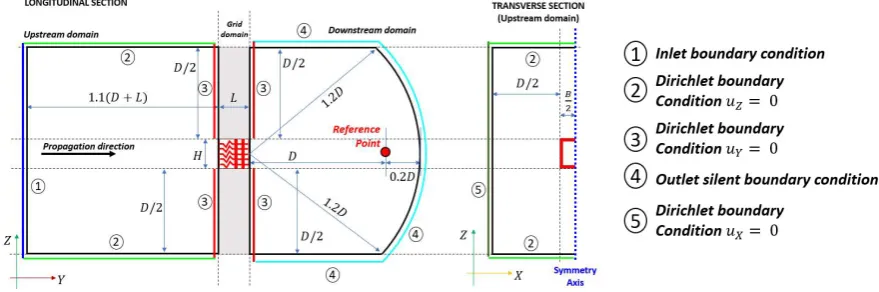
Concerning the development of an appropriate mesh for the upstream and downstream domains, the first step is to determine sufficient dimensions for the meshes of these domains. The proposed approach is described for the cases where both the domains are half-spaces. The case of ducts is more straightforward, because it can be obtained by chopping the dimensions of the half-space to the dimensions of the ducts. The principle for performing the domains dimensioning is presented on Figure 3a. The governing parameter is distance 𝐷 between the grid and a characteristic reference point in the downstream domain, for which the attenuation of the pressure wave is sought (cf. Figure 3). For example, this can be the distance between the grid and the nearest sensitive equipment that should be resistant to the pressure wave. Characteristic distance 𝐷 can be significantly larger than the typical dimensions of the grid.
The dimension of the downstream domain, parallel to the propagation direction, must obviously be at least 𝐷; actually, the domain is prolonged to an additional distance which is around 0.2𝐷, and then a silent boundary condition (non-reflecting outlet boundary condition) is considered. This additional distance
(b)
guarantees that there is no interaction between the outlet boundary and the wave reaching the reference point. Normal to the propagation direction, the downstream domain is prolonged up to a distance equal to 𝐷/2, where a silent outlet is also considered. This guarantees that any spurious reflections on the upper and lower boundaries of the downstream domain will not interfere with the wave reaching the reference point. The same principle is adopted for the out-of-plane direction, (normal to propagation) and the lateral sides are also placed at distance 𝐷/2 from the grid. Finally, anticipating a spherical wave propagation in the downstream half-space, the domain shape is obtained by the intersection of a sphere with radius 1.2𝐷 (or a cylinder, for easiness) with the upper, lower and lateral sides placed at a distance of 𝐷/2 from the grid (cf. Figure 3a). The dimension of the upstream domain is similarly governed by distance 𝐷. Actually, the dimension along the propagation direction must be at least 𝐿 + 𝐷, where 𝐿, the grid dimension parallel to the propagation direction. This guarantees that the refracted wave in the downstream domain will reach the reference point, before any reflected wave in the upstream domain reaches the domain boundary in which the pressure wave is injected via an inlet boundary condition (this is boundary condition (1) on Figure 3); for practical purposes, we take this dimension equal to 1.1(𝐿 + 𝐷). Normal to the propagation direction, the domain dimensions are taken equal to 𝐷/2 for similar reasons as before, so as not to have interference between the reflected waves on lateral sides with the incident wave which is formed just in front of the grid.
Figure 3: Principle for defining the dimensions of upstream and downstream domains
Figure 3 defines the types of boundary conditions that are introduced in the upstream and downstream domains. Boundary condition (1) is an inlet boundary for defining the incident pressure wave. Boundaries (2), (3) and (5) exhibit Dirichlet boundary conditions excluding a velocity of the fluid along the unit normal vector exiting the boundary. Finally, boundary (4) is a silent non-reflecting outlet boundary for simulating the downstream half-space. Following the definition of domain dimensions, the domain discretization must be performed so as to be able to fit exactly with the mesh already defined in the grid domain, in other words the three meshes must be conformal along the two interfaces {upstream / grid} and {grid / downstream}. This explains why the element dimension 𝑒 selected at the grid domain influences the size of the entire model. The efficiency of the calculations is greatly influenced by optimizing the mesh with respect to the following criteria: a) the mesh must be as regular as possible, b) the aspect ratio of the elements must not be larger than a limit for numerical accuracy (typically 3 to 4) and c) the contrast in size between adjacent elements (in particular, parallel to the propagation direction) must be minimal (we accept a bias factor up to 1.005 to 1.01).
DEFINITION OF STATE VARIABLES
- The pressure variation at stagnation state - The density variation at stagnation state
- The equation of state for the air ( perfect gas)
Material velocity and internal energy associated to the shock state are obtained internally within RADIOSS LAW11. The pressure variation at stagnation must anticipate the slight pressure loss δ𝑝 which occurs in passing from stagnation to the shock state. Accordingly, if the absolute pressure peak at the shock state must be exactly equal to 0.110MPa, an inverse calculation allows defining the pressure peak at stagnation which must be 0.1104MPa. The density variation at stagnation is obtained by writing Laplace’s law between the reference state at rest (𝑝 = 0.1MPa, 𝜌 = 1.204kg/m3) and the stagnation state (𝑝 =
0.1104MPa, 𝜌 = ? kg/m3):
𝑝 = 𝑝 → 𝜌 = 𝜌 → 𝜌 =1.292 [kg/m3] (3)
With these definitions at hand, we obtain the pressure and density variations at stagnation as on Figure 4. Material velocity and internal energy are derived directly, without any other additional definition, through the equation of state and the Rankine-Hugoniot equations, which govern the response of the fluid (Hugoniot, 1887). For numerical purposes we suppose that the pressure peak is developed in a very short non-zero time interval, taken equal to 1ms.
Figure 4: Pressure and density variations at stagnation for the definition of inlet boundary conditions
The pressure wave thus injected via the inlet boundary condition is propagated in the upstream domain before reaching the grid. The upstream domain finite element mesh must be regular and fine enough so that the incident wave reaching the grid is indeed the one prescribed and there is no loss in pressure amplitude (10kPa) or elongation of the wave queue (300ms). Finally, for the outlet boundaries, we adopt RADIOSS LAW11, type = 3, which introduces an impedance adjustment at the domain boundaries.
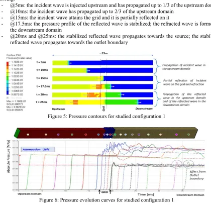
RESULTS - CONFIGURATION 1
We first present the results for studied configuration 1, in which the upstream and downstream domains correspond to ducts of the same section as the grid. The model dimensions are determined so as to study the attenuation for a distance 𝐷 = 5m. This yields a total length in the model (distance between the inlet and the outlet boundaries) of approximately 13m. Nonetheless, it must be noted that for this configuration, the wave propagation in the downstream domain pertains (in a first approximation) to a plane wave without geometric damping (as would be the case for spherical wave propagation). Moreover, there is no reflection in the upstream domain, other than the one occurring in the grid. Therefore, this configuration allows “isolating” the attenuation effect which is only due to the geometric form of the grid, without any effect from possible reflections upstream, or geometric damping downstream.
of the grid. The calculation is pursued for a time interval sufficient so that the incident wave reaches the outlet boundary in the downstream domain, which is approximately 40ms. The selected instants are the following:
- @5ms: the incident wave is injected upstream and has propagated up to 1/3 of the upstream domain - @10ms: the incident wave has propagated up to 2/3 of the upstream domain
- @15ms: the incident wave attains the grid and it is partially reflected on it
- @17.5ms: the pressure profile of the reflected wave is stabilized; the refracted wave is formed in the downstream domain
- @20ms and @25ms: the stabilized reflected wave propagates towards the source; the stabilized refracted wave propagates towards the outlet boundary
Figure 5: Pressure contours for studied configuration 1
Figure 6: Pressure evolution curves for studied configuration 1
A more precise appraisal of the pressure wave propagation can be obtained by plotting the transient evolution of pressure at several characteristic points in the model. The pressure sensors are placed along a longitudinal section passing from the symmetry plane of the grid in all three domains. The position of pressure sensors is presented on Figure 6 together with the corresponding pressure evolution curves. The color of each sensor allows identifying the corresponding curve; actually, this correspondence can simply be established by the sensor position and the characteristic instant at which the pressure wave passes from the sensor. Figure 6 leads to the following conclusions:
- The sensors in the upstream domain reproduce correctly the prescribed incident wave with a characteristic peak equal to 0.11MPa (absolute pressure), a sharp rise to the peak value (~1ms) and a very mild descending branch (extending to 300ms: this can be seen by prolonging the branch until it intersects the horizontal axis).
or even higher (especially for sensors located in front of the steel cylinders, although this is not presented on Figure 6).
- The sensors in the downstream domain reveal the attenuation of the refracted wave with respect to the incident wave. The pressure peaks vary between 0.108MPa and 0.1065MPa with an average value stabilized around 0.1072MPa. This then implies, that the presence of the grid leads to an attenuation of the incident pressure wave between 20% et 35%, with an average value of 28%. This is a direct quantification of the efficiency of a given grid for attenuating a prescribed pressure wave. - For the most remote sensors, close to the outlet boundary, some slight oscillations around the peak value can be observed, which are rapidly attenuated; these may be attributed to a spurious interaction with the outlet boundary.
RESULTS - CONFIGURATION 2
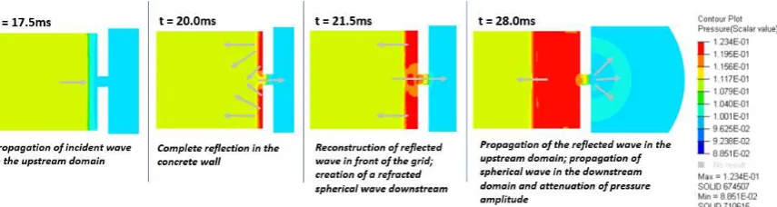
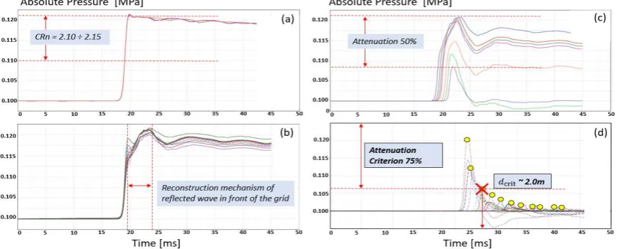
The results related to studied configuration 2, in which half-spaces are considered both for the upstream and downstream domains, highlight: a) the effect of the total reflection of the incident wave in the concrete wall surrounding the grid and b) the effect of spherical wave propagation in the downstream domain leading to a rapid attenuation of peak pressure in the refracted wave. Characteristic contour plots of the pressure field in the entire model are provided for the following instants on Figure 7:
- @17.5ms: the incident wave has almost covered the upstream domain but has not reached yet the concrete wall and the grid
- @20ms: the incident wave is completely reflected in the rigid concrete wall and partially reflected in the grid
- @21.5ms: the reflected wave is reconstructed in front of the grid and attacks the grid - a refracted spherical wave is created in the downstream domain
- @28ms: the reflected wave propagates backwards in the upstream domain; the spherical wave propagates in the downstream domain attenuating the pressure amplitude as it moves away from the grid
Figure 7: Pressure contours for studied configuration 2
Pressure peaks vary between 0.1215MPa in the upstream side and 0.1095MPa in the downstream side. This is equivalent to an attenuation in the refracted wave (with respect to the reflected wave) of approximately 50%, in other words, the refracted wave is almost as strong as the prescribed incident wave because the effects of the reflection on the concrete wall and the attenuation in the grid are almost counter-balanced. It is noticeable that the attenuation effect along the grid is in this case somehow stronger than for studied configuration 1. This may be due to the delay in obtaining the reflected pressures peaks within the grid domain due to the reflected wave reconstruction mechanism. Finally, Figure 8d presents pressure curves at the downstream domain. The obtained pressure peak is attenuated rapidly due to the spherical wave propagation and the ensuing geometric damping. Pressure peaks at different distances from the grid can be used to determine the critical distance 𝑑 satisfying a prescribed attenuation criterion. For example, with reference to Figure 8d, an attenuation of 75% with respect to the reflected wave is achieved at a distance 𝑑 ≥ 2m from the grid.
Figure 8: Pressure evolution curves for studied configuration 2 at different locations: a) at concrete wall, b) in front of the grid, c) along the grid and d) in the downstream domain
CONCLUSIONS
The paper has presented a concise methodology for assessing the efficiency of anti-explosion protective structures using advanced numerical simulation. After discussing the basic principles for a rigorous resolution of the problem of pressure wave propagation through the grid, two typical configurations of a generic grid are studied. Configuration 1 (presence of ducts) allows determining the attenuation effect offered by the geometric form of the grid only. Configuration 2 highlights the effect of the reflected wave on the concrete wall surrounding the grid, the reconstruction of this reflected wave in front of the grid and the spherical wave propagation in the downstream domain with the ensuing strong attenuation with distance due to geometric damping.
REFERENCES
Chatzigogos, C. T., Chauveau, Y. and Nazé, P. A. (2017). Studies on the efficiency of anti-explosion protective structures, Géodynamique & Structure Internal Report N° 35-17.
US Departments of the Army, the Navy and the Air Force. (1990). Structures to resist the effects of accidental explosions. Army TM 5-1300, Navy NAVFAC P-397, Air Force AFR 88-22.
Altair - HyperWorks (2017) An open architecture CAE simulation program.