Iterative Library Subtraction Method for Determining the Contribution of Background Radiation.

(1)

ABSTRACT

MILLER, IAN JAMES. Iterative Library Subtraction Method for Determining the Contribution of Background Radiation. (Under the direction of Dr. Robin P. Gardner).

The analysis of gamma ray spectra is a common task facing many in both academic and

industrial capacities. A widely known method for evaluating spectra of interest is the library

least-squares technique. This method, while very accurate, requires the user to have the

spectral shape of all radioisotopes involved in the unknown spectrum. If a library is missing,

the calculated amounts of each source will be incorrect. This work proposes a method to

apply the principles of spectrum stripping to the unknown spectrum being operated on, with

the aim of determining the spectral shape of any missing libraries. This will be done by

subtracting each known library from the unknown spectrum with a magnitude determined by

a fit to a peak found in both the library and the unknown. The subtraction will continue until

the peak under consideration has been removed from the spectrum. The next known library

will be applied to the residual spectrum, and so on until all known libraries have been

removed. The final residual spectrum is subjected to a threshold method to removed noise; it

can then be used as a library describing other sources of radiation present in the system. This

method produced library spectra that very closely fit to unaccounted for background libraries

in several different unknown spectra. The use of these calculated background libraries in a

library least-squares fit with the known libraries resulted in more accurate results in all tested

spectra. The proposed method could improve the library least-squares technique

significantly, particularly in low energy applications. The ability to produce a background

library without needing to take a separate spectrum could save valuable time and effort for

(2)

(3)

Iterative Library Subtraction Method for Determining the Contribution of Background Radiation

by

Ian James Miller

A thesis submitted to the Graduate Faculty of North Carolina State University

in partial fulfillment of the requirements for the degree of

Master of Science

Nuclear Engineering

Raleigh, North Carolina

2015

APPROVED BY:

_______________________________ _______________________________ Dr. Robin Gardner Dr. Yousry Azmy

Committee Chair

(4)

ii

DEDICATION

To all of those in my life that have allowed me to get to this point; none of this would be

(5)

1

BIOGRAPHY

Ian James Miller was born in Cartersville, GA in 1990 to Dwight and Karen Miller. Being

born into a family with two engineers for parents, it did not take long for science to become a

primary pursuit. During his high school years he was fortunate to attend a technical

conference known as the Air Operated Valve Users Group (AUG) where he was able to meet

several nuclear engineering professionals. Conversing with them about their time at nuclear

power plants or in the nuclear navy, Ian developed an interest in the nuclear sciences. After

graduating from Russell High School in 2008, Ian enrolled at the University of

Tennessee-Knoxville in the nuclear engineering program. He graduated from the honors nuclear

engineering program summa cum laude in 2012, and decided to pursue graduate studies in

nuclear engineering at North Carolina State University. He is currently working on

(6)

2

ACKNOWLEDGMENTS

I’d like to thank my parents, whose guidance has always steered me truly,

My classmates, who made the hard times easier to bear,

My fellow group members at CEAR, whose expertise made this work happen,

(7)

3

LIST OF TABLES

Table 1: NORM Sources of Background ... 26

Table 2: LLS Fitting Results with All Libraries Included ... 33

Table 3: LLS Fitting Results without O Library ... 34

Table 4: Solved Fitting Parameters for Example Spectrum... 45

Table 5: Dampening Constant Application Scheme ... 50

Table 6: Library Multipliers... 56

Table 7: High Background Artificial Spectrum Library Multipliers ... 60

Table 8: Low Background Artificial Spectrum Library Multipliers ... 71

Table 9: Button Source Information ... 83

Table 10: Normalization Constants for Experimental Libraries ... 86

Table 11: Artificial Spectrum Single Peak Subtraction Metrics ... 93

Table 12: Comparison of Convolved to Single Multipliers ... 95

(10)

6

LIST OF FIGURES

Figure 1: Inorganic Scintillation Mechanism ... 21

Figure 2: Photomultiplier Tube ... 23

Figure 3: Elemental Prompt Gamma Libraries for LLS Example ... 31

Figure 4: Example Unknown Spectrum Created by Combination of Example Libraries ... 32

Figure 5: Unknown Spectrum vs. LLS Fit with All Libraries ... 33

Figure 6: Unknown vs. LLS Fit without O Library ... 34

Figure 7: Spectrum Stripping via Elemental Libraries ... 38

Figure 8: Spectrum Stripping Example Libraries ... 39

Figure 9: Unknown Spectrum for Spectrum Stripping Example ... 39

Figure 10: Spectrum Stripping Example Residuals ... 40

Figure 11: Test Spectrum for Method Demonstration ... 42

Figure 12: Fitting Model Plotted Against Peak of Interest ... 44

Figure 13: Result of Attaching a(3) to the H library and Subtracting from Spectrum ... 45

Figure 14: Iterative Subtraction of H Library ... 47

Figure 15: Convergence Behavior ... 48

Figure 16: Realistic Spectrum Example ... 49

Figure 17: Realistic Spectrum Subtraction Convergence ... 49

Figure 18: Damped vs. Undamped Convergence Comparison ... 51

Figure 19: Prompt Gamma and Background Libraries included in Artificial Spectra ... 55

Figure 20: Summation of Chosen Libraries ... 56

(11)

7

Figure 22: High Background Unknown ... 61

Figure 23: High Background H Subtraction ... 62

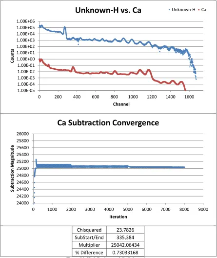
Figure 24: High Background Ca Subtraction... 63

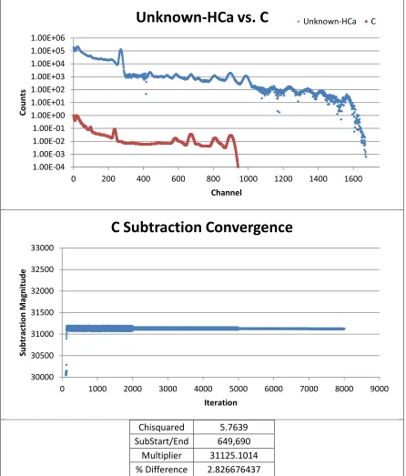
Figure 25: High Background C Subtraction ... 64

Figure 26: High Background S Subtraction ... 65

Figure 27: High Background P Subtraction ... 66

Figure 28: High Background Final Calculated Library Comparison to True Background Library... 67

Figure 29: High Background C and S Convolved Subtraction ... 69

Figure 30: High Background Final Calculated Library Comparison to True Background Library, Convolved Subtraction... 70

Figure 31: Low background Unknown ... 71

Figure 32: Low Background H Subtraction ... 73

Figure 33: Low Background Ca Subtraction ... 74

Figure 34: Low Background C Subtraction ... 75

Figure 35: Low Background S Subtraction ... 76

Figure 36: Low Background P Subtraction ... 77

Figure 37: Low Background Final Calculated Library Comparison to True Background Library... 78

Figure 38: Low Background C and S Convolved Subtraction ... 80

(12)

8

Figure 40: Detection System ... 83

Figure 41: Actual Background for Experimental Spectrum ... 84

Figure 42: Spectrum of all three Button Sources and Background ... 85

Figure 43: Collected Spectrum of Ba133 compared to Library Spectrum of Ba133 ... 86

Figure 44: Collected Spectrum of Co60 compared to Library Spectrum of Co60 ... 87

Figure 45: Collected Spectrum of Cs137 compared to Library Spectrum of Cs137 ... 87

Figure 46: Experimental Spectrum Ba Subtraction ... 89

Figure 47: Experimental Spectrum Co Subtraction ... 90

Figure 48: Experimental Spectrum Cs Subtraction ... 91

(13)

9

LIST OF EQUATIONS

Equation 1: Exponential Decay Law ... 12

Equation 2: Radioactive Decay Constant ... 12

Equation 3: Poisson distribution ... 13

Equation 4: Poisson distribution variance... 13

Equation 5: Gaussian distribution ... 14

Equation 6: Alpha Decay ... 15

Equation 7: Beta Minus Decay ... 15

Equation 8: Beta Plus Decay... 15

Equation 9: Photoelectric Absorption Photoelectron Energy ... 17

Equation 10: Compton Scattering ... 18

Equation 11: Compton Scattered Recoil Electron Energy ... 18

Equation 12: Neutron Elastic Scattering ... 20

Equation 13: Channel Count Rate in Terms of Known Libraries ... 28

Equation 14: Sum of the Squares of Ei ... 28

Equation 15: Series of Least Squares Equations... 29

Equation 16: Series of Least Squares Equations in Matrix Form ... 29

Equation 17: Solution to Least Squares Equations ... 29

Equation 18: Variance of xj ... 29

Equation 19: Reduced Chi-Squared ... 29

Equation 20: Detector Response Function Application ... 36

(14)

10

Equation 22: Threshold Value Determination ... 52

Equation 23: Convolved Peak Fitting Model... 52

Equation 24: Box-Muller Transformation ... 57

(15)

11

Introduction

The analysis of gamma spectra to determine the elemental composition of target

material is a widely used technique. It has the advantage of being non-destructive, and can

be induced in target materials that are not naturally radioactive via neutron activation.

Through the use of pre-generated libraries and techniques such as single peak analysis,

spectrum stripping, or library least squares (LLS) estimations of elemental compositions can

be made. Single peak analysis, while extremely useful for applications using very high

resolution detectors, can fall short in situations where the use of lower resolution detectors is

warranted. The use of elemental library based techniques such as spectrum stripping or

library least squares allows for the use of the information contained across the entire

collected spectrum rather than relying on peak data alone. That is not to say that these library

based methods have no weaknesses. The pre-generated libraries required by these methods

need to be obtained by either time consuming experimental means or computationally heavy

Monte Carlo programming. Assuming those hurdles can be bypassed, there remains a

potential pitfall: that the libraries generated do not cover all sources of radiation present in

the collected unknown spectrum. The composition of the libraries generated to describe a

target unknown material is driven by past operating experience and user input; there is

potential for a source of radiation to not be accounted for due to shifting natural background

or accidental activation during the neutron activation of a target material. Previous attempts

have been made to use the residuals from both library least squares and spectrum stripping to

determine the identity of missing libraries, with a fair amount of success. However the shape

(16)

12

and shape can be extracted but the shape of the continuum often does not agree with the

residuals. This requires a return to the methods used to generate the original libraries. This

can be very time consuming for experimental libraries, assuming that the missing library is

something that can be isolated. For libraries generated through computational means, it may

not be possible to simulate the discovered library, particularly if natural radiation is the

cause. Therefore, methods that can identify a missing library in a library based approach as

well as determine the missing library’s shape would be of value for the field of gamma

spectroscopy.

Radioactive Decay

The basics of radioactive decay described in the following chapters have been sourced from

Radiation Detection and Measurement (Knoll, 2010) and Introductory Nuclear Physics

(Krane, 1988). The phenomenon of radioactive decay was first observed by Antoine Henri Becquerel in 1896. It was noted three years later that this emission of energy is not constant; instead the rate of this decay decreases exponentially with time. This observation leads to the formation of the exponential law of decay, shown below in Equation 1:

Equation 1: Exponential Decay Law

𝑁(𝑡) =𝑁0𝑒−𝜆𝑡

Where N (t) is the number of atoms remaining after time t, N0 is the number of atoms

initially, and λ is the radioactive decay constant, described by Equation 2.

Equation 2: Radioactive Decay Constant

(17)

13

These equations were formulated to take into account two important observations about

radioactive decay: That radioactivity represents changes in the individual atoms of a sample

rather than a change in the sample as a whole, and that the decay is statistical in nature. This

means that it is impossible to know when an individual atom will disintegrate.

Statistical Considerations for Radiation Measurement

Radioactive decay is a random process. As a result, any measurement taken of a

radioactive decay process will be affected by some degree of statistical fluctuation. Given a

constant probability p of “success” or decay, the most general model that can be applied to a

radiation counting experiment is the binomial distribution. However, this model is

cumbersome to use for this application as the number of nuclei considered is always very

large. Assuming that the probability of decay is small for an individual atom and that this

probability is constant it can be shown that the binomial distribution can be simplified to the

Poisson distribution, shown in Equation 3 below, where x is the number of counts observed

in a given time period, 𝑥̅ is the average number of counts observed in that time period, and

P(x) is the probability of observing exactly x number of counts in the given time period.

Equation 3: Poisson distribution

𝑃(𝑥) =(𝑥̅)_𝑥𝑥_!𝑒−𝑥̅

It can be shown that this distribution has a very simple expression for variance in a single

measurement, found in Equation 4.

Equation 4: Poisson distribution variance

(18)

14

This is an important result because it directly relates the number of counts collected during

the measurement of an unknown to the expected variance in the final result; i.e. the more

counts collected the smaller the fractional uncertainty will be. A further simplification to the

Poisson model can be made if the assumption is made that the average number of successes

is large (greater than 25). The result of this assumption is the Gaussian distribution, shown

below.

Equation 5: Gaussian distribution

𝑃(𝑥) = 1

√2𝜋𝑥̅𝑒

−(𝑥−𝑥̅_2𝑥̅)2

The Gaussian distribution is often more convenient that the Poisson distribution as it is a

continuous function rather that a discrete one.

Radioactive Decay Types

A nucleus seeks to decay because it is unstable. This can occur for a number of

reasons, such as a proton/neutron imbalance or currently existing in an excited state. There

are several decay types that nuclei will employ to reach a more stable state. Some examples

are alpha (α), beta (β), and gamma (γ) decay.

Alpha Decays

When a nucleus undergoes alpha decay the unstable nucleus emits an alpha particle in

order to reach a more stable isobar. The alpha particle was shown to be a helium nucleus by

(19)

15

maximizes the kinetic energy the decay can release, which makes the entire process more

favored. The alpha decay process is shown symbolically in Equation 6 below:

Equation 6: Alpha Decay

𝑋_{𝑁 𝛼}→

𝑍

𝐴 _𝑌

𝑁−2 𝑍−2

𝐴−4 ₊ _𝐻𝑒 2 2 4

Where A is the mass number of the atom, Z is the atomic number of the atom, and N is the

neutron number of the atom.

Beta Decays

The goal for beta decay is the same as in alpha decay, but the particle emitted differs.

Instead of nucleons, beta decay emits either an electron or positron. Cases where an electron

is emitted are known as beta minus (β-) decays, positron emission is known as beta plus (β+)

decays. These processes are shown symbolically in Equation 7 and Equation 8.

Equation 7: Beta Minus Decay

𝑋𝑁 𝑍 𝐴

𝛽−

��𝑍+1𝐴𝑌𝑁−1

Equation 8: Beta Plus Decay

𝑋𝑁 𝑍 𝐴

𝛽+

��𝑍−1𝐴𝑌𝑁+1

In both decays, the emission of the beta particle is accompanied by a neutrino. This neutrino

affects the kinetic energy of the beta particle but has no charge.

Gamma Decay

It is fairly uncommon for a nuclear reaction or decay to leave the daughter nucleus in

its ground state. Far more often the end result is an excited daughter nucleus. The primary

method for de-exciting is through gamma decay. While all forms of radioactive decay have

(20)

16

limitations. The primary problem with using alpha and beta particles is that they are quickly

stopped in matter, even air. This limits the range at which the particles can even be detected.

Gamma rays are much more suitable for detection. They can travel much further than the

heavy particles while retaining the energy they were emitted with. If they can be observed in

a suitable manner, it may be possible to determine what isotope emitted them.

Radiation Interaction with Matter

The task of radiation detection would be greatly simplified if all radiation was emitted

in the visual spectrum. Sadly that is not the case. In order to determine anything about

characteristic radiation an interaction with matter that results in something measureable must

occur. This chapter will describe the ways radiation interacts with matter; suitable detection

materials will be discussed in later chapters.

Gamma Ray Interactions

Gamma rays are capable of interacting with matter in a myriad of different ways.

Three of these mechanisms are important for radiation detection, namely photoelectric

absorption, Compton scattering, and pair production. Each functions very differently and is

predominant at different energy ranges.

Photoelectric Absorption

In photoelectric absorption, a gamma ray is absorbed by an atom in the target

material. In its place a photoelectron is ejected. The energy of this photoelectron is

(21)

17

electron. This relationship is shown in Equation 9 below, where Ee- is the energy of the

ejected photoelectron, Eγ is the energy of the incident gamma ray, and Eb is the binding

energy of the electron before ejection.

Equation 9: Photoelectric Absorption Photoelectron Energy

𝐸𝑒−=𝐸𝛾− 𝐸𝑏

This is an important interaction mechanism as it is the only one out of the three primary

interaction mechanisms that results in the complete capture of all the incident energy.

Photoelectric absorption generally has high cross sections at gamma ray energies from 0-300

KeV and for materials with a high Z number.

Compton Scattering

As convenient as it would be for all interaction events to be photoelectric absorption,

many gamma ray energies are much greater than the primary energy range for that

interaction. As incident photon energy increases, the probability of Compton scattering

increases as well. This process, instead of interacting with the entire atom as in photoelectric

absorption, is considered to take place between one electron in the target material and the

incoming gamma ray. The gamma ray is scattered at an angle θ off of its original path. A

portion of the scattering gamma rays energy is transferred to the struck electron, which is

known as the recoil electron. The relationship between the initial (Eγ) and final (Eγ’) gamma

ray energies is shown in Equation 10, where m0c2 is the rest mass of the electron (0.511

MeV). Equation 11 shows the relationship between the energy change of the gamma ray and

(22)

18

Equation 10: Compton Scattering

𝐸𝛾′ = 𝐸𝛾

1 +_𝑚𝐸𝛾

0𝑐2(1−cos𝜃)

Equation 11: Compton Scattered Recoil Electron Energy

𝐸𝑒− =𝐸𝛾− 𝐸𝛾′

Depending on the scattering angle this type of interaction can result in a large amount of

energy imparted to the recoil electron or none at all. This mechanism is present at all

energies, but is the predominant interaction method for gamma rays of energies between

0.5-4 MeV.

Pair Production

Pair production is a process by which a gamma ray with sufficient energy enters the

coulomb field of an atom’s nucleus and in changed into an electron-positron pair. The

energy required for this to happen is twice the rest mass energy of an electron, 1.022 MeV.

The electron created will lose its energy as it travels through the medium until it stops; the

positron will encounter another electron in the target material and annihilate. This is a

process where the positron and electron disappear and two gamma rays with energies equal

to the mass of an electron (0.511 MeV) appear.

Neutron Interactions

For those attempting to ascertain properties of a material via gamma ray spectrum

analysis, it would be convenient indeed if all materials were naturally emitting gamma rays.

Fortunately for the health of all most materials are not significantly radioactive. In order to

(23)

19

outside source. While high energy gamma rays can induce such a state, the most common

mechanism for bulk material activation is through neutron bombardment. The mechanism by

which the neutrons accomplish this depends greatly on the energy of the neutron at the time

of the interaction.

Neutron Capture

The first mechanism for neutron activation of materials is neutron capture. This is an

interaction in which a neutron is absorbed by a nucleus in the target material. After

absorbing the neutron, the nucleus is left in an excited state. It is capable of de-exciting via

many mechanisms, including the emission of a neutron. However the most likely

de-excitation mechanism is through gamma radiation. These gamma rays are emitted at specific

energies determined by the energy level scheme of the target nucleus. This is important

because if the level scheme of a material is known beforehand, gamma rays of certain

energies can be tied to interactions with certain nuclei. The activity of these specific gamma

rays can be used to determine the amount of the nuclei present.

Elastic Scattering

Neutron capture is a very convenient interaction method for inducing gamma activity

in materials where there would otherwise be none. Unfortunately neutron capture is only the

dominant neutron interaction at low energies. The majority of neutron sources produce

neutrons at higher energies where capture is a rare event. The neutrons must be slowed to be

useful; the way that is accomplished is through elastic scattering. Elastic scattering is an

(24)

20

of mass A with energy E; it is then scattered at an angle θ with energy E’. This interaction is

described by Equation 12 below.

Equation 12: Neutron Elastic Scattering

𝐸′

𝐸 =

𝐴2_{+ 1 + 2}_𝐴_cos_𝜃 (𝐴+ 1)2

This relationship shows that the energy lost by the incoming neutron is most heavily

influenced by the mass number of the target nucleus. The heavier the nucleus, the more

elastic collisions must occur to slow the neutron down to thermal energies. In practice, this is

done either by using a hydrogen rich material between the neutron source and the material to

be activated to minimize the number of collisions needed to thermalize the neutrons, or by

using a heavier but denser material to maximize the number of interactions likely to happen

within the intervening material.

Detection Systems

In order for radiation to have any practical use a system must be devised that can

convert the incoming radiation into an electrical signal that can be accepted by today’s signal

processing equipment. This is usually done by the chaining of several signal processing

components together, such as a preamplifier, amplifier, and multichannel analyzer (MCA).

The most important component, however, is the radiation detector itself.

Detector Mechanisms

Simply knowing the ways in which gamma radiation interact with matter is not

(25)

21

incoming gamma rays into something that can be collected by an electronic system.

Fortunately, there are several mechanisms that can accomplish this. The spectra shown later

in this work have all be collected by a sodium iodide (NaI) inorganic scintillator that has

been doped with trace amounts of thallium iodide; the bulk of this section will explain the

mechanism behind this particular detector. The reader should be aware that other systems of

radiation detection exist, such as gas filled or semiconductor detectors. These detectors have

different operating principles but the goal is the same: the conversion of radiation to a

measureable signal.

Inorganic Scintillators

Scintillation radiation detectors seek to transform incident radiation energy into

visible light, which through devices such as a photomultiplier tube can be converted into a

usable electronic signal. This is done by the process of fluorescence, which is the prompt

emission of visible radiation from a substance following its excitement by some means, in

this case, interaction with incoming radiation.

(26)

22

Figure 1 is an illustration of how the excitation process works in inorganic scintillators. The

structure of the conduction and the valence energy bands depends on the crystal lattice of the

scintillation material. The electrons that populate the valence band can be thought of as

bound within the lattice of the crystal, while the conduction band is populated by electrons

that are unbound by this structure. If a gamma ray were to interact with one of the electrons

in the valence band via the mechanisms described in the previous sections it is possible for

that electron to gain enough energy to jump into the conduction band. This creates a “hole”,

or absence of negative charge, in the valence band. This hole will be filled by an electron

from the conduction band; in order for the conduction electron to make the transition to a

lower energy state excess energy is emitted in the form of photons. The wavelength of these

photons is dictated by the band gap. Unfortunately, in a pure crystal, the wavelength of

photons emitted is outside of the visible spectrum and cannot be used as a scintillator. This

can be overcome through doping the crystal with a small amount of impurities known as

activators. The addition of these impurities adds energy levels to the crystal structure

between the conduction an valence bands. Instead of the conduction electron losing all of its

energy at once, creating a photon with an unusable wavelength, the electron can travel

through the energy states of the activator on its way to the valence band. If done properly

this will result in visible light that can form the basis for a scintillation detection system.

However it is important to note that the light emitted from the detection crystal will not be

strong enough on its own to result in a workable signal. Additional multiplication is needed

if the signal generated by the scintillation of the detector is to be discernible over the

(27)

23

Photomultiplier Tubes

The rise of scintillators as radiation detection systems would not have been possible

without the development of the photomultiplier (PM) tube. This device not only transforms

the photons produced by the scintillation crystal into electrons, it is capable of increasing the

magnitude of the resulting signal without adding an undue amount of noise.

Figure 2: Photomultiplier Tube

Figure 2 above shows a simplified structure of the typical photomultiplier tube. There are

two primary components within a PM tube: the photocathode and the electron multiplier.

The photocathode is a negatively charged electrode that is coated in a photosensitive

compound. This ensures that when the photocathode is struck by a photon of light, a

photoelectron will be emitted. The electron multiplication system works by accelerating the

photoelectrons produced by the photocathode. This is done by giving an electrode past the

photocathode a very strong positive charge; this type of electrode is known as a dynode. The

(28)

24

kinetic energy from the acceleration several more electrons will be released. This process

can be repeated several times which will greatly increase the electron yield of the radiation

interaction event.

Preamplifiers

The output from a detector component, regardless of mechanism, is a burst of charge

liberated by the incident radiation. For the scintillation case, with would be the total number

of electrons produced by the photomultiplier tube. The next device in the detection chain is

most commonly a preamplifier. This component seeks to amplify the signal obtained from

the detector before systemic noise clouds it. To do this, the preamplifier is placed as close to

the detector as possible in the signal chain, the aim being to minimize the length of cabling

between the detector and the preamplifier. The preamplifier generally provides no pulse

shaping, and outputs a linear tail pulse to the next device in the detection chain. It should be

noted that in general the signal obtained from a scintillation system is generally quite large

compared to other methods of detection, meaning the amplification of the preamplifier is not

strictly necessary. With that being said it is common practice to include a preamplifier

anyway, as its use will simplify device settings further down the equipment chain.

Amplifiers

The pulses produced by a preamplifier, by design, have a very long tail. This is to

ensure that all of the charge produced by the detection event is collected. However, the tail

also poses a problem for electronic measurement: the information about the radiation event is

(29)

25

overlap the long tail of the previous pulse. As the time between events is random, this makes

the amplitude of the pulse a bad metric for extracting event information. This problem can

be solved by the use of a shaping amplifier. The amplifier shapes the pulses so that the long

tails are eliminated, but the proportionality between the pulse amplitude and the charge of the

radiation interaction event is preserved.

Counting systems

Once a workable pulse shape is obtained, the next task is to determine the objective of

the detection system as a whole. A simple count rate can be obtained by the use of an

integral discriminator, which operates by setting a voltage threshold that the pulse output by

the shaping amplifier must exceed to be counted. If the user desires counting information

about a specific energy range, differential discrimination can be employed. This device,

known as a single channel analyzer (SCA), uses both a high and low voltage threshold. If the

pulse amplitude falls between the two bounds then the pulse is recorded as a count. For

applications that demand the amplitude distribution of pulses from the detector, i.e. spectral

analysis, a multichannel analyzer (MCA) is needed. The simplest way to visualize how an

MCA operates is to imagine several SCAs working in concert. Each SCA, or “channel”, is

active over a certain energy range. If a pulse falls within one of the channels covered by the

MCA, a count for that specific channel is recorded. Once many events have been collected,

(30)

26

Sources of Background Radiation

A constant concern for those attempting to use gamma spectroscopy is that of

background radiation. There are two main sources of background radiation, so called

naturally occurring radioactive materials (NORM) and cosmic radiation (Mitchell, 2008).

NORM represents materials commonly found in the earth or in building materials that

naturally contain radioactive isotopes. There are three isotopes that make up the majority of

NORM background sources: 40K, 232Th, and 238U. The gamma ray energies and intensities

emitted by these isotopes can be found below.

Table 1: NORM Sources of Background

Isotope Energy (keV) Intensity (per decay) 40

K 1460.75 0.1067

232

Th 74.81 0.105

77.11 0.177

238.632 0.433

338.32 0.11257

208

Tl 2614.53 100

238

U 295.24 0.193

351.932 0.376

Note that 208Tl was included as it produces the highest energy gamma ray in the 232Th decay

chain. In fact, this gamma from 208Tl is the highest energy gamma ray produced by

naturally occurring materials; this limits the contribution of NORM sources to a collected

(31)

27

In addition to NORM isotopes, cosmic radiation can also provide a source of

background. This type of background is produced when cosmic radiation interacts with the

earth’s atmosphere, creating secondary radiation such as mesons, electrons, protons,

neutrons, and photons with energies that extend into the hundreds of MeV range. The high

energies this type of background is capable of makes for a much different spectral shape than

NORM sources. NORM sources essentially look like any other gamma ray source, with a

full-energy peak and a continuum behind it. The high energy nature of cosmic radiation,

however, means that few detectors have the size to completely stop an incoming particle.

This means that the spectrum from cosmic radiation is much smoother than NORM, often

lacking a true full energy peak.

A fairly common approach in determining the material composition of a target not

naturally radioactive is to active the target with a source of neutrons. While effective, this

method can also introduce new sources of background into the final spectrum that will need

to be accounted for. The neutrons used to activate the target material will also activate other

materials in the testing environment. A common contributor to the spectrum is the detector

crystal itself, in the form of both activation and prompt gamma rays. Materials surrounding

the detection setup could just as easily become activated and would need to be accounted for.

Gamma rays from the neutron source could also be a contributor, depending on the type of

(32)

28

Library Least Squares applied to Gamma Spectroscopy

The following derivation can be found in greater detail in Analysis of Gamma-Ray

Scintillation Spectra by the Method of Least Squares (Salmon, 1961). For the purposes of

derivation, it will be assumed that the multichannel analyzer used for spectrum collection has

n channels numbered 1…i…n and the spectrum collected is the result of a source that

contains m radionuclides. Individual libraries for these m radionuclides have already been

obtained for the experimental geometry and detection system employed, and will be labeled

1…j…m. The count rate in channel i from library j will be denoted as aij and the total count

rate in channel i will be denoted as bi. Equation 13 shows the relationship between the

recorded count rate and the known libraries, where xj is the multiplier attached to library j

and Ei is random error.

Equation 13: Channel Count Rate in Terms of Known Libraries

𝑏𝑖 =� 𝑎𝑖𝑗𝑥𝑗 +𝐸𝑖 𝑚

𝑗=1

The optimal values of xj can be found by minimizing R, which is the sum of the squares of Ei.

This relationship can be found in below Equation 14.

Equation 14: Sum of the Squares of Ei

𝑅 =� 𝐸𝑖2 𝑛

𝑖=1

= � �𝑏𝑖 − � 𝑎𝑖𝑗𝑥𝑗 𝑚

𝑗=1

�

2 𝑛

𝑖=1

R is minimized by performing a partial derivative with respect to xj and setting the result

equal to zero. Clearly there is one such equation for each channel in the collected spectrum,

(33)

29

Equation 15: Series of Least Squares Equations

� 𝑥𝑗 𝑚

𝑗=1

� 𝑎𝑖𝑘𝑎𝑖𝑗 𝑛

𝑖=1

=� 𝑎𝑖𝑘𝑏𝑖 𝑛

𝑖=1

The series of equations in Equation 15 can be written in matrix form, as shown in Equation

16.

Equation 16: Series of Least Squares Equations in Matrix Form

𝐴𝑥= 𝑦

The solution to Equation 16 can be found below:

Equation 17: Solution to Least Squares Equations

𝑥= 𝐴−1_𝑦

The inverse matrix A-1 can be calculated manually for small values of m, but in the realm of

spectral analysis m is frequently greater than 1000. This necessitates the use of

computational solvers. The variance of xj is given by Equation 18, where [djj]-1 is the

corresponding diagonal elements of the inverse matrix A-1.

Equation 18: Variance of xj 𝑉𝐴𝑅�𝑥𝑗�= _{𝑛 − 𝑚 �𝑑}𝐸 𝑗𝑗�−1

Using this method the best ratio of elements in the mixed source can be determined while

minimizing statistical error and avoiding subjective errors. A convenient method for

determining the quality of the least squares fit to the unknown data is the reduced chi-squared

value, defined below in Equation 19 (Bevington, 2003):

Equation 19: Reduced Chi-Squared

𝜒𝑣2 = 1_{𝑣 �}𝐸𝑖 2

𝜎_𝑖2 𝑛

(34)

30

Where v is the number of degrees of freedom in the dataset and σi2 is the standard deviation

of R. As per Equation 4, σi2can be described by the number of counts in channel i of the

unknown. This process will be performed by a Levenberg–Marquardt (Marquardt, 1963)

based solver known as CURMOD. CURMOD is based on techniques detailed in Bevington

(Bevington, 2003).

One weakness in this method, however, is that all of the radionuclides present in the

collected spectrum need to have a library associated with them. If a major contributor to the

collected spectrum is not included in the least squares solution, the other known libraries will

be forced to include the counts of the missing radionuclide in their computed contributions,

leading to incorrect solutions. In order to demonstrate this effect, a brief example has been

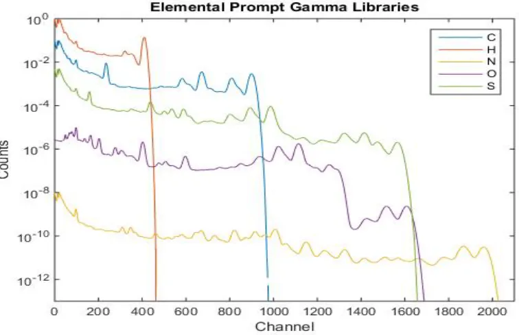
prepared. The author obtained several prompt gamma elemental libraries resulting from the

Monte Carlo simulation of a coal analyzer prototype; specifically these libraries came from

the CEARCPG code developed by Xiaogang Han (Han, 2007). The libraries chosen for this

example are carbon, hydrogen, nitrogen, oxygen, and nitrogen, and can be found in Figure 3

(35)

31

Figure 3: Elemental Prompt Gamma Libraries for LLS Example

The reader should note that the libraries in Figure 3 have been manually spaced so that the

peaks present in each can be easily identified; the actual libraries have all been normalized to

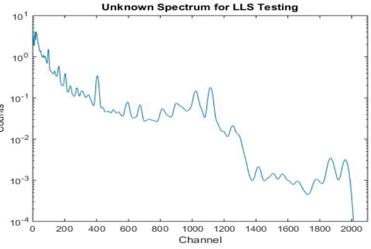
one. These libraries were combined in a 1:1:1:1:1 ratio to create an “unknown” spectrum for

performing a library least squares (LLS) analysis on. This unknown spectrum is shown in

(36)

32

Figure 4: Example Unknown Spectrum Created by Combination of Example Libraries

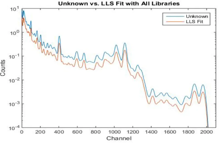
A LLS fit was performed on this unknown including all five libraries using the CEARLLS

code (Gardner R. , 1997); this represents the case where the libraries used in the analysis of

the unknown correctly cover all of the elements present in the unknown. The results of this

fit can be found in Figure 5 and Table 2. Note that an offset has been applied in Figure 5 for

ease of viewing the two datasets; the magnitude of the two is the same across the entire

(37)

33

Figure 5: Unknown Spectrum vs. LLS Fit with All Libraries

Table 2: LLS Fitting Results with All Libraries Included

Library True Library Multiplier

LLS Solved Multiplier

% Area Covered By Library

C 1 1 15.86

H 1 1 14.76

N 1 1 17.14

O 1 1 36.31

S 1 1 15.92

Clearly the fit of the libraries to the unknown results in a satisfactory fit, as was expected.

Figure 6 and Table 3 below show the results of a LLS fit to the same unknown but without

(38)

34

Figure 6: Unknown vs. LLS Fit without O Library

Table 3: LLS Fitting Results without O Library

Library True Library Multiplier

LLS Solved Multiplier

% Area Covered By Library

C 1 0.392717 6.23

H 1 1.12273 16.57

N 1 2.27019 38.92

S 1 1.50377 23.94

As was to be expected, the omission of a contributing library negatively affects the library

(39)

35

Library Generation

In order to utilize the library least squares method for spectral analysis, libraries must

first be constructed. There are two primary methods for library generation: experimental and

calculation. There a benefits and drawbacks to both methods.

Library Generation via Computer Generation

While there are several methods of generating libraries through computer generation,

a method that has risen to prominence is the use of Monte Carlo simulation. The nature of a

Monte Carlo simulation allows for the relatively easy definition of the source and detector

geometry. The primary downside to using a pure Monte Carlo approach is that it is very time

consuming. Each particle needs to be modeled from its “birth” within the radioactive sample

to the resulting pulse of electrons from its interaction within the detector. Tracking a single

gamma ray as it moves through its lifetime is fairly simple; simulating the exact response of

the detector is not. A more practical approach is to use Monte Carlo to determine the extent

of the full energy peak, the Compton continuum, the annihilation photons, and the x-ray

escape peaks. With this data in hand, a detector response function (DRF) is applied to

determine how each incident gamma ray energy will affect the detectors output. As the DRF

is a relatively simple program compared to a full Monte Carlo simulation, this approach can

save a significant amount of time while maintaining a high degree of accuracy. Once the

incident prompt gamma ray spectra for each element in the source of interest has been

simulated through Monte Carlo and the DRF has been determined, it is a fairly simple matter

(40)

36

total number of counts in channel i which have a pulse-height energy Ei, Cjare the counts

incident on channel j in Ej, Dij is the discretized DRF for Ej corresponding to the channel

with Ei, m is the number of energy-count pairs for the element of interest and n is the total

number of channels in each library DRF.

Equation 20: Detector Response Function Application

𝐶𝑖 =� 𝐶𝑗𝐷𝑖𝑗 𝑚

𝑗=1

,𝑖= 1,𝑛

Detector Response Function Generation

There are three main methods of generating DRFs: Experimental, Monte Carlo, and

Semi-empirical. The experimental method entails obtaining the response in matrix form for

several monoenergetic spectra and then interpolating between the known energies to

complete the entire range of energies (Furr, 1968). This method results in spectra that are

closer to elemental library spectra than true DRFs, as they include detector imperfections as

well as shielding in the final result. The downside is that the collection of this information is

extremely time consuming and may not be practical if a very wide range of energies are

required.

The Monte Carlo method (Gardner R. P., 2004) is similar to the experimental method

in that it entails the collection of a large number of monoenergetic spectra and the

interpolation between them; the difference is that these spectra are simulated rather than

collected experimentally. While this minimizes the amount of experimental work that must

be done, care must be taken to appropriately characterize the source-detector system.

(41)

37

The semi-empirical method (Sood, 2004) requires the determination of an analytical

model for separable detector features and uses a least squares fit to a number of

monoenergetic spectra to determine model parameters. This approach requires less

experimental data and can be tailored for individual detectors; the problem is that very little

insight can be gleaned about the actual deposition mechanics within the detector through an

analysis of the analytic model. If the model does not match with experimental data, it can be

difficult to determine why.

Spectrum Stripping

Spectrum Stripping was one of the first attempts to use the library concept to analyze

gamma ray spectra. After the acquisition of elemental libraries that describe the composition

of the unknown, the library with the highest energy peak is identified. This peak is should

exist in the unknown if the libraries adequately describe the unknown and enough counting

time was taken to ensure good counting statistics; assuming that it does, the library

corresponding to this peak is subtracted from the entire unknown spectrum until the highest

energy peak is removed from the system. Once the peak is removed, the library’s

contribution to the unknown is considered to be removed as well. The library with the next

highest energy peak is identified, and the process repeats. This process is shown graphically

(42)

38

Figure 7: Spectrum Stripping via Elemental Libraries

In this figure the unknown spectrum is represented by the dotted lines; the libraries used for

subtraction are shown by dashed lines. In this authors case, the metric used to determine

when a peak was completely removed from the system was a least squares fit of the library

peak to the corresponding peak in the unknown. The multiplier value attached to the library

that produced the lowest chi squared value was applied to the entire library and subtracted

from the unknown spectrum. The solid line represents the reconstruction of the unknown

spectrum by summing all of the elemental libraries times their solved multipliers. Clearly the

method has merit as the result is a very good fit. In more recent years, a study was done by

DiNova on the use of spectrum stripping in cases where not all libraries were initially known

by the user (DiNova, 2011). A test case was constructed of the combination of Cs-137,

(43)

39

9 shows the combination of these libraries with the addition of Poisson noise to simulate a

real collected spectrum.

Figure 8: Spectrum Stripping Example Libraries

(44)

40

The assumption made was that the spectrum was being analyzed without the knowledge that

uranium was present. The contributions of Cs-137 and Co-60 were stripped away using the

methods described above, which resulted in the residuals found below in Figure 10.

Figure 10: Spectrum Stripping Example Residuals

Clearly the analyst would recognize that something was present in the spectrum. However, if

the goal of the analysis was to determine the contribution of all elements present in the

unknown, the next step would be to generate a library for this newfound contributor via the

methods described earlier in this work, such as by experimentation or Monte Carlo

simulation. If an analysis method existed that could result in a usable library for these

(45)

41

Iterative Subtraction Method Development

The primary problem with subtracting library spectra in the areas in which they would be

most effective (i.e. areas with good counting statistics) is that in all but the most simple

spectra the area with favorable counting statistics will contain contributions from other

sources of radiation besides the library up for subtraction. The method of spectral stripping

relied on subtracting a library until a chosen peak was essentially reduced to zero counts,

with the residual spectrum representing the spectrum less the contributions across all

channels of the removed library. This method will clearly not be sufficient if other

contributors exist in the range of channels used to determine if the subtracting library has

been removed; the magnitude of the subtraction will be far greater than the library’s actual

contribution to the spectrum. Therefore, a different metric for library removal needs to be

defined.

Peak Fitting

In order to illustrate the problem at hand and the method used to solve it, refer to Figure 11

(46)

42

Figure 11: Test Spectrum for Method Demonstration

For this example, the unknown spectrum consists of a linear combination of the prompt

gamma ray spectra of hydrogen and carbon. Traditional spectrum stripping would dictate

that the first peak to be operated on would be at the far right end of the spectrum in Figure

11, removing carbon first. However, the magnitude of the hydrogen peak means that if it

could be subtracted first, subsequent subtractions would be subject to far less error. To do

this, the metric for complete subtraction has to be different than simply attaining zero counts

across the peak in question. The first step will be to define a model that describes hydrogen’s

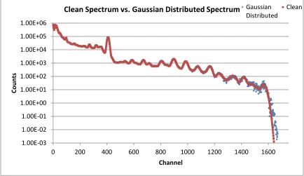
contribution across the range of the peak started at channel 380 and ending at channel 425 as

well as the contribution of other sources of radiation in the same channel range. It can be

shown (Routti, 1969) that a Gaussian distribution can provide a rough approximation of a

photopeak in a gamma ray spectrum. There are features of the photopeak that deviate from

1.00E-04 1.00E-03 1.00E-02 1.00E-01 1.00E+00 1.00E+01 1.00E+02 1.00E+03 1.00E+04 1.00E+05 1.00E+06

0 100 200 300 400 500 600 700 800 900 1000

Co

un

ts

Channel

Example Spectrum

Unknown H

(47)

43

the Gaussian, particularly in the low energy side of the peak in the form of tailing, but in the

interest of the simplest working model a Gaussian will be accurate enough. This portion of

the model will describe the contribution of the library that is being subtracted from the

spectrum, assuming that the peak in the unknown that corresponds to the peak in the library

is not convolved with any other radioisotope peaks. Such convolution will be treated later in

this work. Assuming an unconvolved peak, the other contributions across the peak range will

take the form of a continuum that the library peak sits on top of; this can be reasonably

approximated as a first order polynomial. The entire fitting model can be found in Equation

21 below:

Equation 21: Peak Fitting Model

𝐺𝑎𝑢𝑠𝑠𝑖𝑎𝑛 =𝑎(3)∗exp�−�x−a(1)�

2

2∗a(2)2 �

𝑃𝑜𝑙𝑦𝑛𝑜𝑚𝑖𝑎𝑙=𝑎(4)∗ 𝑥+𝑎(5)

𝑀𝑜𝑑𝑒𝑙= 𝐺𝑎𝑢𝑠𝑠𝑖𝑎𝑛+𝑃𝑜𝑙𝑦𝑛𝑜𝑚𝑖𝑎𝑙

Where a(1) and a(2) are the centroid and standard deviation of the Gaussian, respectively,

and a(3), a(4), a(5) are linear constants. This model conveniently separates the spectral

contribution of the library to be subtracted and all other sources of counts. As such, a new

metric for the subtraction of a library emerges: if the contribution of the Gaussian portion of

this model can be reduced to zero, all that will remain is the contributions of the continuum

underneath the peak. In other words, if the value of a(3) can be minimized, the library is said

to have been removed. Fortunately fitting a peak in a collected spectrum is relatively easy

(48)

44

CURMOD program. The first step toward library removal, once a target library and

corresponding peak in the unknown spectrum has been identified, is to determine the amount

of the library to subtract. An obvious method would be to perform a fit with the model above

and apply the a(3) constant across the target library and then subtracting that library from the

unknown. The results of this operation on the spectrum shown in Figure 11 are shown

below.

Figure 12: Fitting Model Plotted Against Peak of Interest

0 2000 4000 6000 8000 10000 12000 14000 16000

380 390 400 410 420 430 440

Co

un

ts

Channel

Model Fitting Result

(49)

45

Figure 13: Result of Attaching a(3) to the H library and Subtracting from Spectrum

Table 4: Solved Fitting Parameters for Example Spectrum

A(1) 409.0795 A(2) 7.416952 A(3) 13411.89 A(4) -8.15809 A(5) 4412.718

χ^2 1.1829

Figure 12 and Table 4 seem to indicate a very good fit of the model to the targeted peak.

However, Figure 13 shows that the value for a(3) vastly underestimates the magnitude of the

contribution of the hydrogen library to the spectrum. The reason for this is that the library

spectrum describing hydrogen, and indeed every library spectrum, covers more than just the

peak area. When a library is subtracted from the unknown spectrum the continuum on the

1.00E+00 1.00E+01 1.00E+02 1.00E+03 1.00E+04 1.00E+05 1.00E+06

0 100 200 300 400 500 600 700 800 900 1000

Co

un

ts

Channel

(50)

46

low energy side of the peak is altered as well as the peak itself. When the continuum

changes, the model described in Equation 21 will no longer correctly describe the peak in

question. In order to move forward with this idea of subtracting down to the continuum as a

method for library removal an iterative method was adopted.

Iterative Subtraction

As a single round of subtraction was not enough to remove the contribution of a library using

the method as described, a new procedure was developed. A peak in the unknown spectrum

that corresponds to a library spectrum is identified, and the model described in Equation 21 is

applied. The fitted constant a(3) is multiplied across the entire library spectrum, and the

resulting spectrum is subtracted from the unknown spectrum. So far, the method has not

changed from what was described in the previous section. However, the residual of this

subtraction is now taken to be a new unknown spectrum, and the fitting model is applied

across the same channel range as the first fit. A new a(3) constant will be generated and will

be applied across the corresponding library for subtraction again. This process will continue

until the polynomial portion of the model is the primary contributor to the fit across the

channel range. An example of this process can be found in Figure 14 below, where the

(51)

47

Figure 14: Iterative Subtraction of H Library

Clearly after several iterations the contribution of the hydrogen library has been removed

while leaving the contribution of the carbon library intact. The convergence behavior of this

method can be found in Figure 15, where the data points describe the cumulative library

multiplier attached to the hydrogen library in the fit above. There appears to be a point at

which the multiplier attached to the Gaussian portion of the fitting model no longer

contributes to the fit across the peak channel range, as evidenced by the plateau visible in

Figure 15.

1.00E+02 1.00E+03 1.00E+04 1.00E+05 1.00E+06

0 100 200 300 400 500

Co

un

ts

Channel

Iterative Subtraction

(52)

48

Figure 15: Convergence Behavior

When this plateau is reached, the process is said to have converged and the loop exits.

Convergence Dampening

The example spectrum in Figure 11 is a very best case scenario for the application of this

method. There is no statistical noise, there are few radioisotopes involved, and the

radioisotope libraries used for subtraction perfectly describe the radioisotope’s contribution

to the unknown spectrum. These conditions cannot be achieved in realistic testing

conditions, and realistic testing conditions bring additional challenges to applying this

method of subtraction. A possible effect of less than ideal conditions can be shown in the

figures found below.

0 20000 40000 60000 80000 100000 120000

0 100 200 300 400 500

Cu

mu

la

tiv

e L

ib

ra

ry

M

ul

tip

lie

r

Iteration

(53)

49

Figure 16: Realistic Spectrum Example

Figure 17: Realistic Spectrum Subtraction Convergence

1.00E-01 1.00E+00 1.00E+01 1.00E+02 1.00E+03 1.00E+04 1.00E+05

0 500 1000 1500

Co

un

ts

Channel

Realistic Spectrum Subtraction

Unknown S Library 59000 59200 59400 59600 59800 60000 60200

0 1000 2000 3000 4000 5000 6000 7000 8000

Cu mu la tiv e M ul tip lie r M ag ni tu de Iteration

(54)

50

Figure 17 shows that the process is not converging. The magnitude of the Gaussian model is

fluctuating between a positive and negative value without a decrease in magnitude. The final

value is then just determined by the value at the final iteration, which is not acceptable. In

order to combat this, a gradually decreasing dampening constant is introduced. The

dampening constant is applied to the Gaussian magnitude before it is applied to the library

for subtraction, with the goal of lessening the magnitude of the fluctuations of the cumulative

multiplier. This will, given enough iteration, hopefully allow for the convergence of the

process in situations where convergence would otherwise not be possible. This damping

constant is applied in stages as to preserve the initial behavior of the undamped subtraction

process while forcing eventual convergence. This implementation can be found in Table 5

and Figure 18 below.

Table 5: Dampening Constant Application Scheme

Iteration Number

Dampening Constant

0-1999 1

2000-4999 0.5

5000-5999 0.1

6000-6999 0.05

(55)

51

Figure 18: Damped vs. Undamped Convergence Comparison

This figure shows that by applying a dampening constant in this way a converged solution

can be found where there would otherwise be none.

Count Threshold after Subtraction

After all known libraries have been subtracted, it is likely that a band of noise will remain

above any peaks uncovered in the course of applying the method. This band of noise is the

result of differing counting statistics between the library and the unknown spectrum. It is

very likely that the unknown spectrum will have more counts in the areas that a subtracting

library covers; the different amount of counts will result in a different amount of relative

spread between the two data sets. To combat this, a threshold method has been adopted to

determine where statistically significant features begin in the final residual spectrum.

59000 59200 59400 59600 59800 60000 60200

0 1000 2000 3000 4000 5000 6000 7000 8000

Cu mu la tiv e M ul tip lie r M ag ni tu de Iteration

S Subtraction Convergence Comparison

(56)

52

Essentially a threshold value is determined and compared against the number of counts in a

channel. If the threshold value is greater than the number of counts in that channel, the

number of counts in that channel is said to be not significant and is set to zero. If the number

of counts is greater than the threshold value, the number of counts is significant and is left

alone. This procedure is applied to all channels in the residual spectrum. The threshold

value is determined by Equation 22, where yi is the number of counts in channel i and imax is

the maximum number of channels.

Equation 22: Threshold Value Determination

𝑇ℎ𝑟𝑒𝑠ℎ𝑜𝑙𝑑 =�∑_{𝑖𝑚𝑎𝑥}𝑖𝑚𝑎𝑥𝑖=𝑖 𝑦𝑖

Convolved Peak Subtraction

A situation may arise where the highest intensity peak of one library is convolved with a

peak of another library. Applying the subtraction method as described so far will lead to

inaccurate results to a convolved peak, but that does not mean that convolution completely

excludes such a peak from consideration. Instead the fitting model can be modified to fit the

new situation and the subtraction of the convolved library can proceed simultaneously. As

both peaks will be on top of the same continuum, the only change needed to the model

described in Equation 21 is the addition of another Gaussian function to accommodate the

second library peak. The convolved peak fitting function can be found below in Equation 23.

Equation 23: Convolved Peak Fitting Model

𝐺𝑎𝑢𝑠𝑠𝑖𝑎𝑛1 =𝑎(5)∗exp�−�x−a(1)�

2

(57)

53

𝐺𝑎𝑢𝑠𝑠𝑖𝑎𝑛2 =𝑎(6)∗exp�−�x−a(3)�

2

2∗a(4)2 �

𝑃𝑜𝑙𝑦𝑛𝑜𝑚𝑖𝑎𝑙=𝑎(7)∗ 𝑥+𝑎(8)

𝑀𝑜𝑑𝑒𝑙 =𝐺𝑎𝑢𝑠𝑠𝑖𝑎𝑛1 +𝐺𝑎𝑢𝑠𝑠𝑖𝑎𝑛2 +𝑃𝑜𝑙𝑦𝑛𝑜𝑚𝑖𝑎𝑙

This model would be applied across the specified channel range of a convolved peak in the

unknown spectrum, yielding Gaussian multipliers a(5) and a(6). These multipliers would

then be applied to the corresponding libraries and subtracted from the unknown spectrum.

The subtraction would then iterate until only the polynomial had a significant contribution to

the fit; at that point, both libraries involved are said to have been removed. In practice,

however, it was found that CURMOD often struggled to resolve the four nonlinear

parameters involved in this model. This is most like because the peak center (a(1) and a(3))

as well as the standard deviations (a(2) and a(4)) are very similar to each other. After all,

since they are convolved, the centers of the two peaks must be close together, and since they

occupy a very similar energy range the width of the peaks will be similar as well. To

simplify the fit and allow the solver to work with a more linear model a modified procedure

was adopted. The single peak fitting model was applied to both libraries before the

subtraction process began. The peak center as well as the standard deviation in the Gaussian

model was extracted for both of the library peaks. These values were set as constants in the

convolved peak model shown above, replacing variables a(1) through a(4). With the

nonlinear parameters of the Gaussian functions fixed the iterative subtraction is now wholly

(58)

54

scheme was applied to both of the produced library multipliers; this was done in the same

form and for the same function as in the single peak subtraction method.

Artificial Spectra Creation

In order to benchmark these methods, an “unknown” spectrum with known contributions

from established libraries was desired. This would allow for a comparison between the

known magnitude of the library versus the solved magnitude of the library after the

subtraction method was completed. In order to do this five neutron activated prompt gamma

libraries and one natural background library were obtained from the code CEARCPG (Han,

2007). The prompt gamma ray libraries were hydrogen (H), calcium (Ca), carbon (C), sulfur

(S), and phosphorus (P). The natural background library was potassium-40 (k40). These

(59)

55

Figure 19: Prompt Gamma and Background Libraries included in Artificial Spectra

These libraries were chosen simply because they feature a wide range of peaks across a large

number of channels. A combination of these libraries is not meant to approximate a specific

real world scenario; the purpose is to test the subtraction method on a spectrum that is

relatively complex. The first step for creating an artificial “unknown” spectrum is to sum

these libraries together across all channels. The values in Table 6 are applied to their

respective libraries after each library is normalized to their highest value. The magnitudes

found in this table again come from Xiaogang’s work on the CEARCPG code (Han, 2007).

They were chosen simply to have a range of contribution among the included libraries rather

than having equal multipliers. Figure 20 shows the summation of these libraries after they

have been multiplied.

1.00E-06 1.00E-05 1.00E-04 1.00E-03 1.00E-02 1.00E-01 1.00E+00 1.00E+01 1.00E+02 1.00E+03 1.00E+04

0 200 400 600 800 1000 1200 1400 1600

M ag ni tu de Channel

Iterative Library Subtraction Method for Determining the Contribution of Background Radiation.

TABLE OF CONTENTS

LIST OF TABLES

LIST OF FIGURES

LIST OF EQUATIONS

Introduction

Radioactive Decay

Radioactive Decay Types

Radiation Interaction with Matter

Detection Systems

Sources of Background Radiation

Library Least Squares applied to Gamma Spectroscopy

Library Generation

Spectrum Stripping

Iterative Subtraction Method Development

Example Spectrum

Model Fitting Result

Iterative Subtraction

Realistic Spectrum Subtraction

S Subtraction Convergence Comparison

Elemental Libraries Selected for Spectrum Creation