Copyright2000 by the Genetics Society of America
Models for Chromatid Interference With Applications to Recombination Data
F. Teuscher, G. A. Brockmann, P. E. Rudolph, H. H. Swalve and V. Guiard
Research Institute for the Biology of Farm Animals, 18196 Dummerstorf, GermanyManuscript received April 12, 1999 Accepted for publication July 25, 2000
ABSTRACT
Genetic interference means that the occurrence of one crossover affects the occurrence and/or location of other crossovers in its neighborhood. Of the three components of genetic interference, two are well modeled: the distribution of the number and the locations of chiasmata. For the third component, chromatid interference, there exists only one model. Its application to real data has not yet been published. A further, new model for chromatid interference is presented here. In contrast to the existing model, it is assumed that chromatid interference acts only in the neighborhood of a chiasma. The appropriateness of this model is demonstrated by its application to three sets of recombination data. Both models for chromatid interference increased fit significantly compared to assuming no chromatid interference, at least for parts of the chromosomes. Interference does not necessarily act homogeneously. After extending both models to allow for heterogeneity of chromatid interference, a further improvement in fit was achieved.
D
URING meiotic prophase 1 in diploid individuals, involved in a crossover depend in some way on those each chromosome is paired with its homologue. strands involved in neighboring crossovers. Each homologue is duplicated, producing two identicalSubstantial progress has been made in investigating chromatids, the sister strands. A crossover represents an
and modeling the first two components. For these cases event where two nonsister chromatids form chiasmata,
we use the term suppression interference (SI). For SI break, and reunite, enforced by the tight contact and
models, no chromatid interference (NCI) is assumed. the twisting between the chromatids and the subsequent
For recent reviews see Karlin and Liberman (1994) repair mechanism. After meiosis, one of the four
re-andMcPeekandSpeed(1995). The2-model of recom-sulting gametes is randomly chosen for further
inheri-bination (Fosset al.1993;Zhaoet al.1995a) is accepted tance. For clarity we use the term chiasma at the
four-as a satisfying model for positive SI. Negative SI, i.e., strand stage, while the term crossover is used with single
one chiasma enforcing the occurrence of another one, strands or gametes. Hence, from one nonsister strand
can be described, for example, by a negative binomial chiasma, two crossovers result. An example of a meiosis
count distribution for the number of chiasmata. at the four-strand stage is given in Figure 1. It has often
The investigation of CI has not reached the same level been proven that chiasma or crossover events are not
yet. It started in the 1930s when recombination fractions independent. The notion of genetic interference
de-⬎0.5 had been observed. This phenomenon was termed scribes the effect on crossovers of neighboring
cross-pseudolinkage. Models have been developed for data overs. The components of interference are as follows:
exhibiting pseudolinkage (Winge1935;Mather1938). i. Non(complete)randomness in the number of cross- Particularly, Mather found that this phenomenon could overs: The no-interference model applies if the cross- result only from CI. However, little evidence was found over numbers are Poisson distributed. All other for it in diploid organisms. For a review and a test proce-count distributions yield deviations from no interfer- dure, seeZhaoet al.(1995b). Recently,ZhaoandSpeed
ence. (1998, 1999) developed a model for CI. To our
knowl-ii. Non(complete)randomness in crossover locations: edge, an application has not been published so far. The suppression of nearby crossovers has been mod- Summarizing the literature, the general view is that CI eled by nonuniformly distributed locations and by is not evident. This is reflected by widely distributed nonexponentially distributed intercrossover distances mapping software (e.g., CRIMAP) that reduce recombi-with renewal point processes. nation fractions ⬎0.5 to 0.5. Yet, recombination frac-iii. Chromatid interference (CI): The strands actually tions ⬎0.5 are accepted in tetraploids. Recombination
fractions of up to 0.8 have been found in tetraploid fish (Wright et al. 1983). Since ⱕ 0.5 is valid even for
Corresponding author: Friedrich Teuscher, FBN Dummerstorf,
tetraploid species under NCI [see formula (6) withQ⫽ W.-Stahl-Allee 2, 18196 Dummerstorf, Germany.
E-mail: [email protected] 0.25], there is evidence for an action of CI.
Figure 1.—Example of a four-strand-stage meiosis with four chi-asmata and resulting gametes. A pair of vertically linked, solid circles indicates a chiasma: two nonsister strands break and re-combine. Shaded circles denote resulting crossovers on the ga-metes. Open circles define loci with observable genotypes. Two-neighbored chiasmata are called complementary if they have no strand in common, reciprocal if they have two strands, and diago-nal if they have one strand in common.
Hence, CI cannot be excluded, either from a theoreti- To develop a CI model that takes this into account and gives additional information compared to the CI() cal point of view, or from empirical evidence. It
there-fore appears to be helpful to derive alternative models model, we assume here that CI acts only in the neighbor-hood of a chiasma. Then a complementary chiasma pair to the existing model ofZhaoandSpeed(1998), either
to increase the evidence for CI in diploids or to strengthen is modeled by a parallel nonsister strand pair;i.e., two complementary chiasmata occur close to one site. As the conviction that there is none. The objective of the
present study was to develop a model allowing parallel mentioned above, this would lead to the phenomenon of double crossovers. On the other hand, nearby recip-nonsister strand chiasmata, which could not arise under
high SI if one assumes suppression on all four strands, rocal chiasmata would look like sister strand chiasmata since they would seldom lead to observable recombina-and sister strrecombina-and chiasmata, which also have not been
modeled so far but could play a role at high SI. In tions. Thus we also allow sister strand chiasmata. Let us again consider the question whether suppres-analyzing a number of recombination data sets we found
evidence for SI and CI. Until now heterogeneity of inter- sion of nearby chiasmata acts on all four strands or only on those involved in the chiasma. So far an answer to ference has not been investigated. We incorporated CI
heterogeneity into both CI models and obtained further this question is not known. If we assume the highest amount of suppression in the first case, then the maxi-improvement in fit.
mum average suppression distance is 0.5 M since within this distance the next chiasma must appear. In the latter METHODS
case, the maximum average suppression distance is 1 M, since a chiasma on the complementary strands could
The CI() model ofZhaoandSpeed(1998):Zhao
andSpeed(1998) treatedWeinstein’s (1936) andMath- restore the needed expected number of chiasmata. In this way, complementary pairs are enforced, which can er’s (1938) approach of modeling CI by introducing a
parameter that defines the probability that a strand be considered to be parallel from a model point of view. Additionally, sister strand chiasmata have been observed involved in a chiasma is also involved in the following
chiasma. From this, the probabilities for complemen- repeatedly. Although they are invisible to the observer of recombinations, they influence the location of neigh-tary, diagonal, and reciprocal chiasma pairs (cf.Figure
1) are (1⫺ )2, 2(1⫺ ), and2, respectively. Under bored nonsister strand chiasmata if suppression is a property of nonsister as well as sister strand chiasmata. NCI these are1⁄
4,1⁄2, and1⁄4. Thus ⬎0.5 indicates an
increased and ⬍0.5 a reduced amount of reciprocal Therefore, they must be taken into account.
Assume the four-strand stage of meiosis of diploids. chiasma pairs compared to complementary pairs. The
force of CI is assumed to be independent of the distance We define a chiasma site to be a location on a chromo-some, where strands break and reunite. Let P be the between the neighbored chiasmata. For the underlying
SI process the2-model of recombination was chosen; probability that exactly two nonsister strand chiasmata occur at a chiasma site and S that one or two sister i.e., suppression of nearby chiasmata is working on all
four strands. This model here is called CI(). strand chiasmata occur. Consequently, 1⫺P⫺Sis the probability that exactly one nonsister chiasma appears
The CI(Q) model allowing sister strand and parallel
nonsister strand chiasmata:Jarrellet al.(1995) found at the chiasma site. The chance of a chiasma site
produc-ing a crossover on a gamete is thenQ⫽(1⫹P⫺S)/2. an increased occurrence of four-strand double
cross-overs at the centromere of bovine chromosome 23. For We assumed that there are no dependencies between different chiasma sites;i.e., for this, NCI is assumed. all models of SI derived for the four-strand bundle, such
x and an appropriate recombination fraction . The will result from a chiasma on a random gamete with probabilityQ⫽2/a.Therefore, forQ⫽1, (5) coincides relationship betweenxandis given by the map
func-tion(x). Letc⬘i(x) be the probability thaticrossovers with the map function of the two-strand stage,
appear between the loci on the gamete. Then for the
expected number of crossovers (x)⫽
兺
∞
i⫽0
c⬘2i⫹1(x)⫽ 1 2
冦
1⫺兺
∞
i⫽0 (⫺1)ic
i(x)
冧
; (8)x⫽
兺
∞i⫽1
ic⬘i(x) (1)
cf. Bailey (1961). For Q ⫽ 0.5, with the four-strand stage of diploids,
must be valid. A crossover results from a chiasmata site
with probabilityQ.Under the given assumptions, with (x)⫽{1⫺ c
0(x)}/2 (9)
ci(x) being the probability that the interval carries i
found byMather (1938), and for Q ⫽ 0.25 with the chiasma sites, we determine
eight-strand stage of tetraploids.
The map function for CI(Q): Recall the 2-model
c⬘i(x)⫽
兺
∞
j⫽i
P(icrossovers|jchiasma sites)cj(x)
of recombination. The chiasma formation process is described by a stationary renewal process, where the ⫽ Qi
兺
∞
j⫽i
冢
j
i
冣
(1⫺ Q)j⫺ic
j(x). (2) intercrossover distances follow a 2-distribution with 2(m ⫹ 1) d.f. For the theory derived by Zhao et al. From the expectation condition (1) at the gamete level (1995a) the model ofFoss et al. (1993) of the same we obtain the requirement process is helpful. In this model the locationsCof so-called gene conversions are assumed to be uniformly x⫽
兺
∞
j⫽0
兺
ji⫽0
冢
j i冣
iQi(1⫺
Q)j⫺i
cj(x)⫽Q
兺
∞
j⫽1
jcj(x) (3) and independently distributed on a scaley.Their values
follow a Poisson distribution. By this, not every gene conversion C leads to a nonsister strand chiasma Cx. at the four-strand stage. An obvious consequence is the
One realizedCxis followed bymgene conversionsCo, limitation of the distance given as
from which no crossovers result. Afterward the nextCx xⱕ nQ (4) is produced. Parametermis the interference parameter,
m⫽0 indicates no interference. The probability of no ifn is the maximum number of chiasmata. From the
crossovers was determined to be fact that a recombination results from an odd number
of crossovers,
c0(x)⫽
兺
mi⫽0
冢
1⫺ i
m⫹1
冣
hi(y), (10) (x)⫽12
冦
1⫺兺
∞i⫽0
(1⫺ 2Q)i
ci(x)
冧
withhi(y)⫽e⫺yyi/i!. The relationship between the scale
ywith the genetic scalexisy⫽ 2(m⫹ 1)xunder NCI. ⫽1
2
冦
兺
∞i⫽0
(1⫺ (1⫺2Q)i)c
i(x)
冧
(5) The application of the CI(Q) model is based on theassumption that an eventCxrepresents a chiasma site can be evaluated for the recombination fraction. Its now, which leads to a crossover on a gamete with
proba-upper bounds are bility Q. The relation between the model scale y and
the genetic scalex then changes to y ⫽ (m ⫹ 1)x/Q. (x)ⱕ0.5 forQⱕ0.5, (6)
The probability of the crossover numberi⫽0 is given
and by (10) and those fori⫽ 1, 2, . . . are found to be
(x)ⱕ Q forQ ⬎0.5. (7)
ci(x)⫽hi(m⫹1)(y)⫹
兺
mj⫽1 j
m⫹1{h(i⫺1)(m⫹1)⫹j(y)⫹h(i⫹1)(m⫹1)⫺j(y)} Remember that Q ⬍ 0.5 indicates the preference of
(11) reciprocal pairs andQ⬎0.5 the preference of
comple-mentary chiasma pairs. By this we have a CI model that formⱖ1 andci(x)⫽hi(y) form⫽0. The map function
can be evaluated via (5) now. As for the map function is in concordance with the finding ofMather(1938)
that a recombination fraction exceeding a half may only of the CI() model ofZhaoandSpeed(1998), recombi-nation fractions⬎0.5, monotone decreasing parts, and be the result of an enlarged number of complementary
chiasmata. even wave shapes may arise. Form→ ∞andQ⫽1, the
map function converges to the periodic map function Before we can apply the model we have to define the
chiasma site distribution {ci(x)}. As done byZhao and of complete interference investigated by Teuscher
(1997). Speed(1998), we use the 2-model of recombination.
The combined model is denoted with CI(Q). Note that form⫽0 (Haldane’s model) the CI parame-terQdoes not influence the map function if 0⬍Qⱕ Note that (5) can be viewed as a general formula
for an arbitrary strand stage of meiosis under NCI. A 1 holds. This can be proved by solving (3) and (5) with {ci(x)} following the Poisson distribution.
The distribution of recombination patterns for CI(Q): fit the data, the models for heterogeneous CI are used. If these models are significantly better than the homoge-To find the theoretical distribution {␥(i)} of the
multilo-cus recombination pattern i⫽ (i1, i2, · · · ,ir) for the neous CI models, one source of the heterogeneity is
gametes, whereik⫽1 indicates a recombination andik⫽ proved. If the data still do not fit satisfactorily,
heteroge-0 indicates absence of recombination between markersk neous SI appears to act and is subject to further investi-andk⫹1 on a randomly chosen gamete, we can follow gations: We divide the chromosome and start with the the Appendix ofZhaoet al.(1995a). Besidesy⫽(m⫹ analysis of all pairs of adjacent intervals. For each pair 1)x/Q, a difference is the chance of schiasmata in an there are four possible recombination patterns, (0, 0), interval to produce a recombination, which is (1⫺(1⫺ (1, 0), (0, 1), and (1, 1), to which we have to fit the 2Q)s)/2 now, derived from (5). Thus we obtain
observations. Since the sample size is known, three equa-tions have to be solved. Practice shows that this can be realized by the two genetic distances to be estimated ␥(i)⫽ 1
m⫹11⬘M1M2· · ·Mr1 (12) and by the introduction of one parameter to estimate SI. Following this, we analyze all triples of adjacent intervals, with Mj⫽R∞k⫽0(1 ⫹(⫺1)ij(1⫺2Q)k)Dk(yj)/2 andyj ⫽
then the quadruples, etc. (m⫹ 1)xj/Q. Dk(y) is the (m ⫹ 1) ⫻ (m⫹ 1) matrix
The test criterion for the fit of the models to real
whosei,jth entry ise⫺yy(m⫹1)k⫹j⫺i/((m⫹1)k⫹j⫺ i)!.
data: Commonly, the multilocus concept of Weeks et
Definition of models CI(Qi) and CI(i) for the
investi-al.(1993) is used to analyze recombination data. For a
gation of heterogeneity of interference:Assume the
fre-directly observable multilocus recombination pattern, quent case that a model of a crossover formation process
the criterion of fit is the log-likelihood does not fit recombination data. Two reasons might
explain this. The data set may be too small or unreliable,
lnL⫽max
冢
兺
i
n(i)ln(␥(i))
冣
, (13) or the model might not be appropriate. For the lattercase we have to check the assumptions. In all models
wheren(i) is the observed number and␥(i) is the theo-created so far the real process is assumed to be
homoge-retical probability of recombination patterni.Ther⫹ neous over the whole chromosome. This is not
necessar-1 markers are assumed to be ordered, with genetic dis-ily true. We therefore investigate heterogeneous
proc-tances between each consecutive pair of markersx1,x2, esses. Our hypothesis is that when finding the same
· · · ,xr.The maximum has to be determined by varying
degree of interference for two adjacent or overlapping
the genetic distances and the parameters of the model. regions of a chromosome, the model is applicable if it
Haldane’s no-interference model is nested in the fits both parts together. On the other hand, we cannot
2-model of recombination, representing the NCI expect a model to fit data for a certain region if it
model. The NCI model is nested in both models for already failed for a part of it, or if different parts of it
homogeneous CI;i.e., a likelihood-ratio test can be ap-show different characteristics of interference.
plied to test whether CI is acting or not. Also, the CI(Q) From a preliminary analysis we concluded that
inter-and CI() models are nested in the CI(Qi) and CI(i)
ference is likely to act heterogeneously. A generalization
models, respectively, and we can test whether CI hetero-of the CI models to regard heterogeneous SI appears
to be difficult. We propose the incorporation of CI het- geneity is significant. To compare two nested models, a erogeneity. We therefore introduce CI parameters into likelihood-ratio test is applied. Following the asymptotic the models that may vary between different parts of theory, twice the difference of the two log-likelihoods the chromosome. For the CI(Q) model, like the CI() of the models is2-distributed with the difference of the model ofZhaoandSpeed(1998), we assign CI parame- number of parameters being the degrees of freedom. tersQiandito intervalsi, which does not change the In the application of the models for heterogeneous
theory in any significant way. These models are denoted CI, the interval-wise CI parametersQˆiandˆi,i⫽1, · · ·,r,
by CI(Qi) and CI(i), respectively. However, the two- have to be estimated. To obtain a statement for intervali,
whether deviations from NCI are significant, we com-locus recombination fractions then are not only a
pare the complete models for each i with the model function of the distance between the loci but of their
restricted byQi ⫽0.5 ori⫽0.5, respectively.
locations. To ensure 0 ⱕ Qi,i ⱕ 1 during numerical
We evaluate the quality of a fitted model by compar-calculations, we fit auxiliary variablesziand putQi,i⫽
sin2(z
i). ing its log-likelihood value with the ideal log-likelihood
value theoretically achievable by an unknown model Given a recombination data set we apply the following
procedure. First we fit Haldane’s no-interference that fits the observed gamete distribution exactly; i.e., for this model,␥(i)⫽n(i)/NwithN⫽Rin(i) is valid. If
model, then a NCI model like the2-model of
recombi-nation for positive SI or alternatively the negative bino- twice the difference of the two log-likelihoods is smaller than the 1 ⫺ ␣-quantile of the 2-distribution with 1 mial map function for negative SI. To test CI vs. no
For this case we use the phrase that the model fits the val analysis are displayed in theappendix, Tables A4 and A5. A significant improvement over the models data.
assuming homogeneous CI is observed.
Application to the data of Weinstein (1936): The
RESULTS
seven-locus Drosophila data ofWeinstein(1936) have also often been analyzed (e.g., Zhao et al. 1995a). All
Application to the data ofMorganet al.(1935):The
nine-locus Drosophila data ofMorganet al.(1935) have models applied here yield a significant gain in fit when compared to nested models. The log-likelihood for Hal-often been used to compare crossover formation models
(seeMcPeekandSpeed1995). The data have not been dane’s model is⫺56,394.3 and that of the CI() model under absence of interference (m ⫽ 0, ˆ ⫽ 0) is fitted well by any model. Compared with the ideal
log-likelihood of⫺36,899.5, we obtained lnL⫽ ⫺37,956.6 ⫺55,096.2. The results for the other models are shown in Table 1. Again we see that the effect of SI is larger for Haldane’s no-interference model, lnL⫽ ⫺36,987.1
for the NCI model (2-model of recombination with than that of CI. However, both effects and even the effect of heterogeneous CI are significant. To investigate mˆ ⫽ 4; similar to the gamma model of McPeek and
Speed1995), and lnL⫽ ⫺37,122.1 for the CI() model the heterogeneity of SI we analyzed adjacent intervals by the NCI model. We obtainedmˆ ⫽4 for the first two under absence of SI (m⫽0,ˆ⫽0). We find significance
for the effects of both SI and CI. Models CI(Q) and intervals and mˆ ⫽ 5, 4, 3, and 3 for the subsequent interval pairs. All models fitted the data. Analysis of CI() are not significantly better than the NCI model,
thus proving that homogeneous CI is not evident in three neighboring intervals with the NCI, CI(Q), and CI() models led to the results summarized in the ap-addition to SI. Models CI(Qi) and CI(i) with ln L⫽
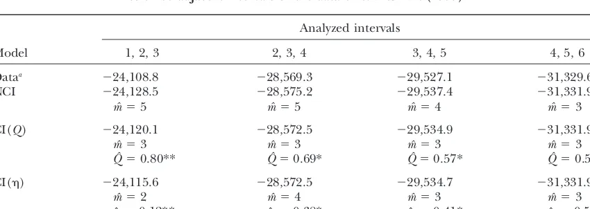
⫺36,943.0 and lnL⫽ ⫺36,950.0, respectively, however, pendix, Table A6. Only the triple of intervals (4, 5, 6) almost fitted. This was supported by the same interfer-yield a highly significant gain in fit when considering
heterogeneous CI. To investigate the heterogeneity of ence strength of m ⫽ 3 in intervals (4, 5) and (5, 6). Different interference strengths in neighboring inter-SI, we analyzed first pairs of adjacent intervals by the
NCI model. We obtained mˆ ⫽ 4 for the first pair and vals led to triples not fitting. At the first, second, and third triples we found significant improvement of the mˆ ⫽ 5, 4, 3, 4, 4, and 2 for the subsequent interval
pairs. All models fitted the data. The analysis of three NCI models by the CI models. Both models suggest an increased occurrence of complementary chiasmata. neighboring intervals with the NCI, CI(Q), and CI()
models gave the results summarized in theappendix, Then we analyzed the quadruples of adjacent inter-vals. The results are shown in theappendix, Table A7. Table A1. Only the triple of intervals (5, 6, 7) could be
fitted well. This was supported by the same interference For the first and second quadruples we again found a highly significant improvement over the NCI model. strengthm⫽ 4 in intervals (5, 6) and intervals (6, 7).
Different SI strengths at neighbored interval pairs led We applied the CI(Qi) and CI(i) models to the
four-interval case and compared the results with the six-to triples not fitting. At the first and second triples we
found significant improvement of the NCI model by interval analysis (Table A8). Some significant improve-ments over the models of homogeneous CI were found. the CI models. Both models suggest an increased
occur-rence of complementary chiasmata. Application to the data of Blank et al.(1988):The recombination data ofBlanket al.(1988) on chromo-Then we analyzed the quadruples of intervals. The
results are shown in theappendix, Table A2. For the some 12 of mice have been used repeatedly for investiga-tions on the phenomenon of interference (Weekset al. first quadruple, termed the “five-locus data ofMorgan
et al.(1935)” in the literature, and the second and fourth 1994; LinandSpeed 1996). The analysis of the whole data set led to results shown in Table 2. Furthermore, quadruple a highly significant improvement over the
NCI model is evident. Deviating from the former conclu- we obtained lnL⫽ ⫺564.67 for fitting Haldane’s model and lnL⫽ ⫺547.63 for fitting CI() under absence of sions, both CI models indicate a significant effect of
dominating reciprocal chiasmata at quadruple (4, 5, 6, SI (m⫽0,ˆ⫽0);i.e., the effects of SI (lnL⫽ ⫺547.12 under NCI) and CI nearly agree. Both effects are sig-7). However, from quadruples onward, no model fits
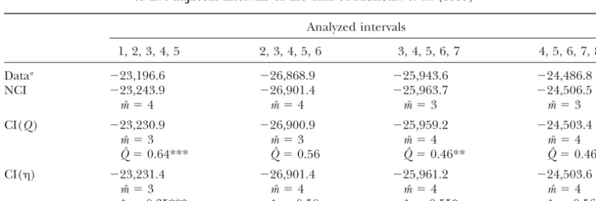
the data. The analysis of the quintuples (Table A3) nificant compared to assuming no interference. The CI(Q) and CI() models are significantly better than underlines the tendency of the telomeric part to carry
an increased number of reciprocal chiasma pairs. The the NCI model, which was so far viewed to fit best (Lin and Speed 1996). For the CI(Qi) model we obtained
dominance of complementary chiasma pairs at the
cen-tromere region is still visible. The analysis of six neigh- the best fit formˆ ⫽6,Qˆ1 ⫽0.19,Qˆ2⫽· · ·⫽ Qˆ5 ⫽1, Qˆ6 ⫽ 0.87, and Qˆ7 ⫽ 0.72. This model is significantly boring intervals with the CI(Q) model indicates the
same result. There, model CI() showed significance better than the NCI model but not significantly better than the model for homogeneous CI. OnlyQˆ1 differs only at the telomeric part. With seven or eight intervals,
no improvements over the NCI model are found. significantly from 0.5. For the CI(i) model we obtained
the best fit formˆ ⫽ 1,ˆ1 ⫽ ˆ2 ⫽ 1, and ˆ3 ⫽ · · ·⫽ We applied the CI(Qi) and CI(i) models to the
TABLE 1
Observed gamete counts of the data ofWeinstein(1936) and counts expected for the2-model under NCI and under different models for chromatid interference
Expected
NCI: CI(Q): CI(): CI(Qi): CI(i):
mˆ ⫽4, mˆ ⫽3, mˆ ⫽4, mˆ ⫽3, mˆ ⫽3,
Gamete Observed Q⫽ ⫽0.5 Qˆ ⫽0.60 ˆ⫽0.46 Qˆi(see Table 9) ˆi(see Table 9)
(0, 0, 0, 0, 0, 0) 12,776 13,054.0 12,771.5 12,759.5 12,777.5 12,774.3
(1, 0, 0, 0, 0, 0) 1,407 1,267.7 1,310.9 1,313.7 1,393.0 1,402.8
(0, 1, 0, 0, 0, 0) 2,018 1,893.7 1,964.7 1,959.7 2,072.9 2,049.6
(0, 0, 1, 0, 0, 0) 1,976 1,793.0 1,856.1 1,850.9 1,910.3 1,912.9
(0, 0, 0, 1, 0, 0) 3,378 3,324.0 3,428.3 3,426.0 3,394.1 3,416.9
(0, 0, 0, 0, 1, 0) 2,356 2,404.5 2,474.4 2,484.0 2,366.2 2,360.2
(0, 0, 0, 0, 0, 1) 2,067 2,101.8 2,179.5 2,178.1 2,053.0 2,063.5
(1, 1, 0, 0, 0, 0) 9 9.0 11.8 8.6 7.6 11.5
(1, 0, 1, 0, 0, 0) 16 44.6 45.1 42.5 29.1 21.1
(1, 0, 0, 1, 0, 0) 142 211.1 189.4 199.3 150.3 144.6
(1, 0, 0, 0, 1, 0) 198 226.2 206.0 211.7 196.6 196.9
(1, 0, 0, 0, 0, 1) 206 214.0 211.2 202.1 213.0 209.2
(0, 1, 1, 0, 0, 0) 11 13.8 18.0 13.4 9.7 9.4
(0, 1, 0, 1, 0, 0) 136 170.7 163.0 163.6 126.5 135.0
(0, 1, 0, 0, 1, 0) 261 274.7 243.7 259.0 241.4 249.2
(0, 1, 0, 0, 0, 1) 318 305.7 285.9 286.5 295.8 294.2
(0, 0, 1, 1, 0, 0) 42 47.9 54.1 46.8 47.6 48.7
(0, 0, 1, 0, 1, 0) 148 163.6 148.9 156.4 165.6 166.6
(0, 0, 1, 0, 0, 1) 212 247.6 221.9 232.6 242.2 245.0
(0, 0, 0, 1, 1, 0) 123 88.2 93.3 85.5 130.5 110.7
(0, 0, 0, 1, 0, 1) 315 270.2 247.1 256.4 298.6 291.9
(0, 0, 0, 0, 1, 1) 59 43.1 47.9 41.2 56.1 61.2
(1, 1, 0, 1, 0, 0) 3 0.7 0.8 0.6 0.4 0.7
(1, 1, 0, 0, 1, 0) 1 1.2 1.4 1.1 0.9 1.3
(1, 1, 0, 0, 0, 1) 2 1.4 1.7 1.2 1.1 1.6
(1, 0, 1, 0, 1, 0) 3 3.8 3.5 3.4 2.4 1.8
(1, 0, 1, 0, 0, 1) 3 6.0 5.3 5.2 3.6 2.7
(1, 0, 0, 1, 1, 0) 10 4.8 4.6 4.3 5.1 4.3
(1, 0, 0, 1, 0, 1) 15 16.1 12.9 14.0 12.5 11.9
(1, 0, 0, 0, 1, 1) 1 3.9 3.9 3.4 4.3 5.0
(0, 1, 1, 1, 0, 0) 1 0.3 0.4 0.3 0.2 0.2
(0, 1, 0, 1, 1, 0) 2 3.3 3.5 3.0 4.0 3.6
(0, 1, 0, 1, 0, 1) 10 12.2 10.6 10.8 10.2 10.7
(0, 1, 0, 0, 1, 1) 1 4.6 4.4 4.0 5.0 6.2
(0, 0, 1, 1, 0, 1) 5 3.0 3.2 2.7 3.6 3.6
(0, 0, 1, 0, 1, 1) 5 2.5 2.6 2.2 3.1 3.9
(0, 0, 0, 1, 1, 1) 1 1.1 1.4 1.0 1.9 2.3
(1, 1, 1, 1, 0, 0) 1 0.001 0.002 0.0005 0.0004 0.001
(1, 1, 1, 0, 0, 1) 1 0.004 0.008 0.004 0.003 0.004
lnL ⫺54,850.1a ⫺54,950.2 ⫺54,931.8 ⫺54,935.8 ⫺54,890.0 ⫺54,887.8
aIdeal case: theoretical and observed distributions agree.
homogeneous model CI(). Estimates ˆ3, ˆ6, and ˆ7 Compared to the ideal log-likelihood of lnL⫽ ⫺270.96, only the CI(i) model fitted the data, indicating
substan-differ significantly from 0.5. From the estimates of the
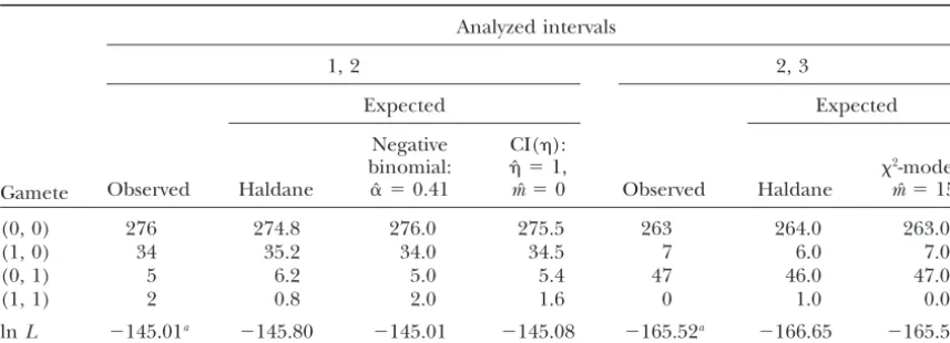
heterogeneity parameters we hypothesize that the prob- tial heterogeneity in the first three intervals. The results of analyzing the first adjacent pairs with NCI models lem is to fit the first three intervals and the last six.
Analysis of the first three intervals gave lnL⫽ ⫺277.62 are shown in theappendix, Table A9. For the first two intervals, the resultmˆ⫽0 suggests that Haldane’s model for the NCI model (m ⫽ 1), ln L ⫽ ⫺276.72 for the
CI() model (ˆ ⫽ 0.23,mˆ ⫽ 1), ln L ⫽ ⫺276.95 for fitted best. The model fitted the data. We also applied the negative binomial map function and fitted the data the CI(Q) model (Qˆ ⫽1,mˆ ⫽1), and lnL⫽ ⫺272.28
TABLE 2
Observed gamete counts of the data ofBlanket al.(1988) and counts expected for the2-model under NCI and under different models for chromatid interference
Expected
NCI: CI(Q): CI(): CI(Qi): CI(i):
mˆ ⫽6, mˆ ⫽2, mˆ ⫽2, mˆ ⫽6, mˆ ⫽1;
Gamete Observed Q⫽ ⫽0.5 Qˆ ⫽1 ˆ⫽0.15 Qˆi(see text) ˆi(see text)
(0, 0, 0, 0, 0, 0, 0) 148 159.3 148.0 148.4 149.4 146.4
(1, 0, 0, 0, 0, 0, 0) 27 30.8 32.9 31.9 26.1 31.7
(0, 1, 0, 0, 0, 0, 0) 5 6.0 6.6 6.5 6.1 5.8
(0, 0, 1, 0, 0, 0, 0) 45 36.6 41.5 41.7 43.1 43.7
(0, 0, 0, 1, 0, 0, 0) 4 3.2 3.6 3.6 3.7 3.8
(0, 0, 0, 0, 1, 0, 0) 6 4.8 5.4 5.4 5.6 5.7
(0, 0, 0, 0, 0, 1, 0) 24 20.3 22.9 23.3 24.1 24.1
(0, 0, 0, 0, 0, 0, 1) 47 39.3 44.8 46.1 46.9 46.5
(1, 1, 0, 0, 0, 0, 0) 2 0.01 0.02 0.04 0.2 0.7
(1, 0, 0, 0, 0, 1, 0) 2 2.1 1.3 1.0 1.9 0.9
(1, 0, 0, 0, 0, 0, 1) 5 7.2 4.5 3.3 5.6 3.5
(0, 0, 1, 0, 0, 0, 1) 2 3.6 2.6 2.3 1.2 2.3
lnL ⫺531.92a ⫺547.12 ⫺543.28 ⫺542.93 ⫺538.60 ⫺536.21
aIdeal case: theoretical and observed distributions agree.
than positive interference. For the second pair we found negative or absent SI at the centromere region and high SI at the telomeric part of the chromosome for the data lnL ⫽ ⫺165.52 for mˆ ⫽ 15. Although not significant
compared to Haldane’s model, a strong positive inter- of Blanket al.(1988).
The results on CI also differ between data sets. We ference seems to act.
For intervals 2–7 the NCI model already fits the data therefore conclude that no general rules for interfer-(mˆ ⫽ 29). We evaluated ln L ⫽ ⫺430.03, which was ence heterogeneity exist. Using the data ofMorganet highly significantly better than Haldane’s model (lnL⫽ al.(1935) andWeinstein(1936) we found an increased ⫺452.48). For comparison, the ideal log-likelihood was amount of complementary chiasmata at the centromere ⫺428.96. region. For the data ofMorganet al.(1935) we addition-ally found an increased amount of reciprocal chiasma pairs at the telomeric part of the chromosome. This is DISCUSSION particularly evident from the results for the CI(Q)
model and could result from sister strand chiasmata. A long-known reason for the occurrence of chiasmata
Using the data of Blank et al. (1988) we proved an is to help organize meioses by fixing strands. On the
intensification of complementary chiasma pairs that are other hand, it turned out that molecular strategies of
concentrated mainly in the telomeric part. The findings inheritance play an important role in the biological
for the centromere weakly indicate either an increased process of evolution. It is not clear if or how chiasmata
amount of reciprocal chiasmata or simply negative SI. are involved in this process. Only trivial statements can
One should note that Morgan et al. (1935) and be made, such as negative or absence of genetic
interfer-Weinstein(1936) examined the same chromosome of ence increases genetic variability on the gametes more
the same species. It is of particular interest that the first than high positive interference. The investigation of
five loci and the seventh locus were identical. Compar-meiotic processes with particular sets of recombination
ing Tables A1 and A6, A2 and A7, A4 and A8, and A5 data is only one but an important step in contributing
and A8, we indeed observe a congruence of parameter knowledge in this area.
estimates and interference behavior. Both models for The NCI models routinely used in mapping today
CI behaved similarly. Therefore it is not clear whether reflect only SI. We have proved that, as well as SI, CI and
CI works better at small or large distances. We note that even interference heterogeneity may play an important
numerically the CI(Q) model is about five times faster role in meiosis. We found evidence for heterogeneous
than the CI() model. SI and CI. The SI heterogeneity differed among the
We have shown that chromatid and suppression inter-three data sets considered. While we found positive,
ference are not completely separable. Especially, posi-slightly varying intermediate SI for the data ofMorgan
Brockmann, G. A., C. S. Haley, U. Renne, S. A. Knottand M. amount of complementary chiasma pairs and negative
Schwerin,1998 QTLs affecting body weight and fatness from SI by an enlarged amount of reciprocal chiasma pairs. a mouse line selected for extreme high growth. Genetics150:
368–381. For the data ofMorgan et al. (1935) and Weinstein
Foss, E., R. Lande, F. W. StahlandC. M. Steinberg,1993 Chiasma (1936), SI dominates CI, while for the data ofBlanket interference as a function of genetic distance. Genetics133:681– al. (1988) both kinds of interference have the same 691.
Jarrell, V. L., H. A. Lewin, Y. DaandM. B. Wheeler,1995 Gene-strength. However, separation would be easier if we were
centromere mapping of bovineDYA,DRB3, andPRLusing sec-dealing with data exhibiting obvious deviations from ondary oocytes and first polar bodies: evidence for four-strand NCI, such as recombination fractions⬎0.5 or decreas- double crossovers betweenDYAandDRB3.Genomics27:33–39. Karlin, S.,andU. Liberman,1994 Theoretical recombination proc-ing recombination fractions for increasproc-ing distances.
esses incorporating interference effects. Theor. Popul. Biol.46: Let us consider the data ofBlanket al.(1988). The data 198–231.
do not cover the whole chromosome. The maximum Lin, S.,andT. P. Speed,1996 Incorporating crossover interference into pedigree analysis using the2model. Hum. Hered.46:315– recombination fraction is 0.498. The CI models fitted
322.
suggest that the recombination fractions would exceed Mather, K.,1938 Crossing over. Biol. Rev.13:252–292.
McPeek, M. S.,and T. P. Speed,1995 Modeling interference in 0.5 if the whole chromosome had been investigated. If
genetic recombination. Genetics139:1031–1044. this is not true, the gain in fit explained with CI is an
Morgan, T. H., C. B. Bridges andJ. Schultz,1935 Report of artifact. Then we would have proved that the2-model
investigations on the constitution of the germinal material in relation to heredity. Carnegie Inst. Wash.34:284–291. of recombination is not appropriate to the data, but
Teuscher, F.,1997 On the multilocus feasibility of map functions that another chiasma formation process is adequate, for depending crossover placement rules. Arch. Tierz.40:179– and may be a nonstationary renewal one. However, 191.
Weeks, D. E., M. LathropandJ. Ott,1993 Multipoint mapping our experience with mouse markers (Brockmann et
under genetic interference. Hum. Hered.43:86–97.
al. 1998) shows that recombination fractions can ex- Weeks, D. E., J. OttandM. Lathrop,1994 Detection of genetic
ceed 0.5. interference: simulation studies and mouse data. Genetics136:
1217–1226. From our results and from the indications found for
Weinstein, A.,1936 The theory of multiple-strand crossing over. CI acting in tetraploids, we conclude that chromatid Genetics21:155–199.
interference is likely to act. We encourage geneticists Winge, O¨ .,1935 On the possibility of cross-over percentages over 50. C. R. Lab. Carlsberg21:60–76.
to be aware of recombination fractions exceeding
one-Wright, J. E., K. Johnson, A. HollisterandB. May,1983 Meiotic half and that the phenomenon of interference hetero- models to explain classical linkage, pseudolinkage, and chromo-some pairing in tetraploid derivative salmonid genomes, pp. 239– geneity should not be ruled out.
260 inIsozymes: Current Topics in Biological and Medical Research, The authors are indebted to Dr. T. P. Speed, Phillip Huff, and two Vol. 10, Genetics and Evolution. A. R. Liss, New York.
anonymous reviewers for numerous suggestions on an earlier version Zhao, H.,andT. P. Speed,1998 Stochastic modeling of the crossover process during meiosis. Commun. Stat. Theory Methods 26: of the manuscript.
1557–1580.
Zhao, H.,andT. P. Speed,1999 On a Markov model for chromatid interference, pp. 1–37 inStatistics in Molecular Biology and Genetics, edited byF. Seillier-Moiseiwitsch.American Mathematical
So-LITERATURE CITED ciety, Providence, RI.
Zhao, H., T. P. SpeedandM. S. McPeek,1995a Statistical analysis Bailey, N. T. J.,1961 Introduction to the Mathematical Theory of Genetic
of crossover interference using the Chi-square model. Genetics Linkage. Oxford (Clarendon) University Press, Oxford.
139:1045–1056. Blank, R. D., G. R. Campbell, A. CalabroandP. D’Eustachio,
Zhao, H., M. S. McPeekandT. P. Speed,1995b Statistical analysis 1988 A linkage map of mouse chromosome 12: location ofIgh of chromatid interference. Genetics139:1057–1065.
and effects of sex and interference on recombination. Genetics
APPENDIX TABLE A1
Log-likelihoods and estimated parameters for different models of interference fitted to three adjacent intervals of the data ofMorganet al.(1935)
Analyzed intervals
Model 1, 2, 3 2, 3, 4 3, 4, 5 4, 5, 6 5, 6, 7 6, 7, 8
Dataa ⫺12,745.2 ⫺15,650.7 ⫺15,049.3 ⫺17,531.2 ⫺15,511.3 ⫺13,918.1
NCI ⫺12,753.6 ⫺15,659.7 ⫺15,051.4 ⫺17,534.5 ⫺15,512.4b ⫺13,921.9
mˆ ⫽5 mˆ ⫽5 mˆ ⫽3 mˆ ⫽3 mˆ ⫽4 mˆ ⫽4
CI(Q) ⫺12,750.7 ⫺15,655.1 ⫺15,051.4 ⫺17,534.5 ⫺15,512.4b ⫺13,920.9
mˆ ⫽3 mˆ ⫽3 mˆ ⫽3 mˆ ⫽3 mˆ ⫽4 mˆ ⫽3
Qˆ ⫽0.87* Qˆ ⫽0.73** Qˆ ⫽0.50 Qˆ ⫽0.50 Qˆ ⫽0.50 Qˆ ⫽0.60
CI() ⫺12,749.5 ⫺15,654.2 ⫺15,051.4 ⫺17,534.4 ⫺15,512.4b ⫺13,920.8
mˆ ⫽2 mˆ ⫽2 mˆ ⫽3 mˆ ⫽3 mˆ ⫽4 mˆ ⫽3
ˆ ⫽0.09** ˆ⫽0.25** ˆ ⫽0.51 ˆ ⫽0.50 ˆ⫽0.50 ˆ⫽0.36
Significantly better than NCI model. *P⬍0.05; **P⬍0.01.
aIdeal case: theoretical and observed distributions agree. bModel is not significantly improved.
TABLE A2
Log-likelihoods and estimated parameters for different models of interference fitted to four adjacent intervals of the data ofMorganet al.(1935)
Analyzed intervals
1, 2, 3, 4 2, 3, 4, 5 3, 4, 5, 6 4, 5, 6, 7 5, 6, 7, 8
Dataa ⫺18,751.3 ⫺20,099.7 ⫺21,820.1 ⫺21,655.2 ⫺18,343.3
NCI ⫺18,776.2 ⫺20,125.1 ⫺21,827.3 ⫺21,670.9 ⫺18,348.3
mˆ ⫽5 mˆ ⫽4 mˆ ⫽3 mˆ ⫽4 mˆ ⫽4
CI(Q) ⫺18,762.0 ⫺20,120.6 ⫺21,827.2 ⫺21,667.7 ⫺18,347.1
mˆ ⫽2 mˆ ⫽3 mˆ ⫽4 mˆ ⫽4 mˆ ⫽3
Qˆ ⫽1.0*** Qˆ ⫽0.61** Qˆ ⫽0.44 Qˆ ⫽0.45* Qˆ ⫽0.57
CI() ⫺18,761.0 ⫺20,120.5 ⫺21,827.3 ⫺21,667.3 ⫺18,347.8
mˆ ⫽3 mˆ ⫽3 mˆ ⫽3 mˆ ⫽3 mˆ ⫽3
ˆ⫽0.24*** ˆ ⫽0.37** ˆ⫽0.50 ˆ⫽0.58** ˆ⫽0.41
Significantly better than NCI model. *P⬍0.05; **P⬍0.01; ***P⬍0.001.
aIdeal case: theoretical and observed distributions agree.
TABLE A3
Log-likelihoods and estimated parameters for different models of interference fitted to five adjacent intervals of the data ofMorganet al.(1935)
Analyzed intervals
1, 2, 3, 4, 5 2, 3, 4, 5, 6 3, 4, 5, 6, 7 4, 5, 6, 7, 8
Dataa ⫺23,196.6 ⫺26,868.9 ⫺25,943.6 ⫺24,486.8
NCI ⫺23,243.9 ⫺26,901.4 ⫺25,963.7 ⫺24,506.5
mˆ ⫽4 mˆ ⫽4 mˆ ⫽3 mˆ ⫽3
CI(Q) ⫺23,230.9 ⫺26,900.9 ⫺25,959.2 ⫺24,503.4
mˆ ⫽3 mˆ ⫽3 mˆ ⫽4 mˆ ⫽4
Qˆ ⫽0.64*** Qˆ ⫽0.56 Qˆ ⫽0.46** Qˆ ⫽0.46*
CI() ⫺23,231.4 ⫺26,901.4 ⫺25,961.2 ⫺24,503.6
mˆ ⫽3 mˆ ⫽4 mˆ ⫽4 mˆ ⫽4
ˆ⫽0.35*** ˆ ⫽0.50 ˆ ⫽0.55* ˆ ⫽0.56*
Significantly better than NCI model. *P⬍0.05; **P⬍0.01; ***P⬍0.001.
TABLE A4
Estimated chromatid interference parametersQˆiand obtained log-likelihoods for the five- and
nine-locus analyses of the data ofMorganet al.(1935) with model CI(Qi)
Qˆifor intervali
lnL
Analyzed intervals (mwith best fit) i⫽1 i⫽2 i⫽3 i⫽4 i⫽5 i⫽6 i⫽7 i⫽8
1, 2, 3, 4 ⫺18,757.3* (3) 0.51 1a 1a 0.52
2, 3, 4, 5 ⫺20,102.2** (3) 1a 1a 0.51 0.37
3, 4, 5, 6 ⫺21,824.2 (3) 0.90a 0.46 0.40 0.70a
4, 5, 6, 7 ⫺21,662.0* (4) 0.34 0.51 0.46 0.82
5, 6, 7, 8 ⫺18,344.5 (3) 0.36 0.73 0.54 0.30
1, 2, 3, 4, 5, 6, 7, 8 ⫺36,943.0** (3) 0.52 1a 1a 0.51 0.34a 0.73a 0.49 0.34
1, 2, 3, 4, 5, 6, 7, 8 ⫺36,944.4** (4) 0.35 0.88a 0.99a 0.42 0.38 0.55 0.53 0.23
Significantly better than model for homogeneous interference. *P⬍0.01; **P⬍0.001.
aEstimate differs significantly from 0.5 (P⬍0.05).
TABLE A5
Estimated chromatid interference parametersˆiand obtained log-likelihoods for the five- and
nine-locus analyses of the data ofMorganet al.(1935) with model CI(i)
ˆifor intervali
lnL
Analyzed intervals (mwith best fit) i⫽1 i⫽2 i⫽3 i⫽4 i⫽5 i⫽6 i⫽7 i⫽8
1, 2, 3, 4 ⫺18,756.2* (2) 0 0.14a 0.08a 0.20a
2, 3, 4, 5 ⫺20,102.3** (2) 0 0.07a 0.19a 0.40a
3, 4, 5, 6 ⫺21,825.9 (3) 0 0.39 0.55 0.50
4, 5, 6, 7 ⫺21,661.2* (4) 1 0.98a 0.58a 0.54
5, 6, 7, 8 ⫺18,346.9 (3) 1 0.40 0.37a 0.45
1, 2, 3, 4, 5, 6, 7, 8 ⫺36,953.0** (3) 0 0.29 0.13a 0.26a 0.46 0.50 0.52 0.50
Significantly better than model for homogeneous interference. *P⬍0.01; **P⬍0.001.
aEstimate differs significantly from 0.5 (P⬍0.05).
TABLE A6
Log-likelihoods and estimated parameters for different models of interference fitted to three adjacent intervals of the data ofWeinstein(1936)
Analyzed intervals
Model 1, 2, 3 2, 3, 4 3, 4, 5 4, 5, 6
Dataa ⫺24,108.8 ⫺28,569.3 ⫺29,527.1 ⫺31,329.6
NCI ⫺24,128.5 ⫺28,575.2 ⫺29,537.4 ⫺31,331.9
mˆ ⫽5 mˆ ⫽5 mˆ ⫽4 mˆ ⫽3
CI(Q) ⫺24,120.1 ⫺28,572.5 ⫺29,534.9 ⫺31,331.9
mˆ ⫽3 mˆ ⫽3 mˆ ⫽3 mˆ ⫽3
Qˆ ⫽0.80** Qˆ ⫽0.69* Qˆ ⫽0.57* Qˆ ⫽0.50
CI() ⫺24,115.6 ⫺28,572.5 ⫺29,534.7 ⫺31,331.9
mˆ ⫽2 mˆ ⫽4 mˆ ⫽3 mˆ ⫽3
ˆ⫽0.12** ˆ⫽0.38* ˆ⫽0.41* ˆ ⫽0.50
Significantly better than NCI model. *P⬍0.05; **P⬍0.001.
1459 Chromatid Interference TA BL E A 7 Log-likelihoods and estimated parameters for different mod els of inter feren ce fi tte d to fo u r adj acent inter vals of the data of Weinstein (1936) Analyzed intervals 1, 2, 3, 4 2 , 3 , 4 , 5 3, 4, 5, 6 a ⫺ 35,471.3 ⫺ 38,214.4 ⫺ 39,280.8 ⫺ 35,513.0 ⫺ 38,239.2 ⫺ 39,304.1 mˆ ⫽ 5 mˆ ⫽ 4 mˆ ⫽ 4 Q ) ⫺ 35,491.8 ⫺ 38,234.1 ⫺ 39,297.5 mˆ ⫽ 3 mˆ ⫽ 3 mˆ ⫽ 3 Q ˆ ⫽ 0.71** Q ˆ ⫽ 0.60* Q ˆ ⫽ 0.55** ) ⫺ 35,494.0 ⫺ 38,235.2 ⫺ 39,297.1 mˆ ⫽ 3 mˆ ⫽ 4 mˆ ⫽ 3 ˆ ⫽ 0.29** ˆ ⫽ 0.46* ˆ ⫽ 0.45** Significantly better than NCI m odel. * P ⬍ 0.01; ** P ⬍ 0.001. a Ideal case: theoretical and observed distributions agree. TABLE A8
Estimated chromatid interference parametersQˆiandˆiand obtained log-likelihoods for the five- and seven-locus analyses
of the data ofWeinstein(1936) with models CI(Qi) and CI(i)
CI(Qi) CI(i)
Qˆifor intervali ˆifor intervali
Analyzed
intervals lnL(mˆ) 1 2 3 4 5 6 lnL(mˆ) 1 2 3 4 5 6
1, 2, 3, 4 ⫺35,488.6 (3) 0.56 0.92a 0.78a 0.58 ⫺35,483.9**(3) 0 0.33 0.15a 0.31a
2, 3, 4, 5 ⫺38,220.6**(3) 0.58 1 0.56a 0.45a ⫺38,221.9* (3) 0 0.20a 0.31a 0.45a
3, 4, 5, 6 ⫺39,286.6**(3) 1 0.60a 0.41 0.77a ⫺39,289.9* (3) 0 0.28a 0.44a 0.47
1, 2, 3, 4, 5, 6 ⫺54,890.0**(3) 0.57 0.97a 0.69a 0.62a 0.38a 0.96a ⫺54,887.8**(3) 0 0.30 0.16a 0.31a 0.45a 0.49
Significantly better than model for homogeneous interference. *P⬍0.01; **P⬍0.001.
TABLE A9
Observations of the first two interval pairs of the data ofBlanket al.(1988) with expected numbers obtained by fitting different models
Analyzed intervals
1, 2 2, 3
Gamete
Expected Expected
Observed
Negative CI():
binomial: ˆ ⫽1, 2-model:
Haldane ␣ˆ⫽0.41 mˆ ⫽0 Observed Haldane mˆ ⫽15
(0, 0) 276 274.8 276.0 275.5 263 264.0 263.0
(1, 0) 34 35.2 34.0 34.5 7 6.0 7.0
(0, 1) 5 6.2 5.0 5.4 47 46.0 47.0
(1, 1) 2 0.8 2.0 1.6 0 1.0 0.0
lnL ⫺145.01a ⫺145.80 ⫺145.01 ⫺145.08 ⫺165.52a ⫺166.65 ⫺165.52