Signal Processing using Wavelets for Enhancing Electronic Nose Performance

(1)

Abstract

PHAISANGITTISAGUL, EKACHAI. Signal Processing using Wavelets for Enhancing Electronic Nose Performance. (Under the direction of Dr. H. Troy Nagle.)

In recent years, many new technologies of electronic devices that mimic the mammalian olfactory system, electronic noses (e-noses), have been developed in many research institutions and commercial organizations around the world. These devices have been used in a wide range of applications such as food and beverage quality, environmental monitoring, medical diagnosis. Over the past decade, many researchers have spent a great deal of effort improving e-nose performance and also extended the use of the e-nose devices, not only for discriminating or classifying different odor samples, but also for quantifying an ingredient of a given odor sample.

(2)

SIGNAL PROCESSING USING WAVELETS FOR ENHANCING

ELECTRONIC NOSE PERFORMANCE

by

EKACHAI PHAISANGITTISAGUL

A dissertation submitted to the Graduate Faculty of North Carolina State University

In partial fulfillment of the Requirements for the Degree of

Doctor of Philosophy

ELECTRICAL ENGINEERING

Raleigh, NC 2007

APPROVED BY:

___________________________ ___________________________ Charles E. Smith, Ph.D. Mark White, Ph.D.

(3)

Biography

(4)

Acknowledgements

First of all, I would like to express my sincere appreciation to Dr. H. Troy Nagle, the chairman of my advisory committee. This work would have not been at all possible without his guidance and advice. He introduced me to an electronic nose device which inspired my interest to further enhance its performance in this dissertation. He has provided me not only academic guidance but also constant caring and encouragement. In addition, his expertise and experience as a professional engineer are valuable to accomplish my research.

I would like to thank the other three members of my committee, Dr. Charles E. Smith, Dr. Edward Grant, and Dr. Mark White. Their suggestions and advices during my Ph.D. endeavor were always helpful. I would also extend my appreciation to Dr. Hyeokho Choi who taught and inspired me to apply a wavelet theory on my research. I’m indebted to Dr. Susan Schiffman for letting me perform data acquisition of odor mixture on her electronic nose system.

(5)

List of Tables

Table 2-1. Details of the dataset ……….20

Table 2-2. Odor class identity ………20

Table 2-3. Classification performance results of Bacteria dataset ……….25

Table 2-4. Classification performance results of Coffee dataset ………...26

Table 2-5. Classification performance results of Soda dataset ………..27

Table 3-3. Forward sensor subset selection’s results of Bacteria dataset ………..54

Table 3-4. Backward sensor subset selection’s results of Bacteria dataset ………55

Table 3-5. GA sensor subset selection’s results of Bacteria dataset ………..56

Table 3-6. Forward sensor subset selection’s results of Coffee dataset ……….57

Table 3-7. Backward sensor subset selection’s results of Coffee dataset ………..58

Table 3-8. GA sensor subset selection’s results of Coffee dataset ……….59

Table 3-9. Forward sensor subset selection’s results of Soda dataset ………60

Table 3-10. Backward sensor subset selection’s results of Soda dataset ……….61

Table 3-11. GA sensor subset selection’s results of Soda dataset ………62

Table 4-3. Summary of each classifier algorithm ………..85

Table 4-4. Results of classifier selection performance for each odor type dataset based on 5-fold cross-validation ………87

Table 4-5. Results of classification performance based on 5 fold-cross validation ………...91

Table 5-1. Description of mixture odor dataset ………109

(9)

List of Figures

Figure 1-1. Illustration of the location of the olfactory epithelium of a human …………2 Figure 1-2. Illustration of human olfactory system ………...3 Figure 1-3. Typical block diagram of an electronic nose ………..5 Figure 2-1. A series of responses of sensors no. 1 and 15 to a specific coffee

sample ………..11 Figure 2-2. The block diagram of Machine Olfaction ……….11 Figure 2-3. An acquisition process of an electronic nose ………14 Figure 2-4. (a) The sensor response and error bar plots for a particular coffee

class of 44 samples of sensor no: 12, (b) The sensor response and error bar plots for a particular coffee class of 44 samples of sensor

no: 14 ………15 Figure 2-5. Windowed time slicing based on Bell-shaped kernel ………...16 Figure 2-6. Multilevel wavelet decompositions ………..17 Figure 2-7. (a) Example of sensor responses of a particular coffee class, (b) DWT

of sensor responses based on “db2” ……….17 (c) DWT of sensor responses based on “Haar”, (d) DWT of sensor

responses based on “Biorthogonal 1.3” ………18 Figure 2-8. Flow diagram of the experimental procedure ………...19 Figure 2-9. PCA projection of Bacteria classes after feature compression based

on DWT- db2-level4 ……….22

Figure 2-10. PCA projection of Coffee classes after feature compression based on

DWT- db2-level4 ………..23

Figure 2-11. PCA projection of Soda classes after feature compression based on

DWT- db2-level4 ………..23

Figure 3-1. Typical block diagram of an electronic nose ………34 Figure 3-2. (a) A two-channel filter bank, (b) Mulitlevel two-channel filter

(10)

banks ………38

Figure 3-4. (a) Example of sensor responses of a particular coffee class, (b) 4th-DWT of sensor responses based on “db2” ………39

Figure 3-5. Flowchart of general procedure of feature subset selection ……….41

Figure 3-6. Block diagrams of filter feature subset selection (FSS) and wrapper FSS methods ………44

Figure 3-7. A procedure of sequential forward sensor subset selection ……….45

Figure 3-8. A procedure of a sequential backward sensor subset selection ………46

Figure 3-9. A procedure of the Genetic algorithm (GA) ………47

Figure 3-10. An example of GA operation for sensor subset selection ………49

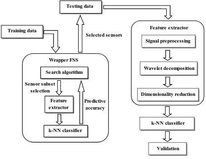
Figure 3-11. A flow diagram of sensor subset selection with wrapper method …………50

Figure 3-12. Windowed time slicing based on Bell-shaped kernel ………...51

Figure 3-13. PCA projection plots of Bacteria dataset (a) Full set of 15 sensors, (b) GA sensor subset selection (sensor no: 6) ………..63

Figure 3-14. PCA projection plots of Coffee dataset (a) Full set of 15 sensors, (b) GA sensor subset selection (sensor no: 6) ………..64

Figure 3-15. PCA projection plots of Soda dataset (a) Full set of 15 sensors, (b) GA sensor subset selection (sensor no: 4, 7, 10, and 15) ………64

Figure 4-1. The Multiple Classifier System (MCS) algorithm ………72

Figure 4-2. The proposed classifier selection algorithm ……….74

Figure 4-3. Illustration of odor-type signatures of the training data subset (the coffee odor signatures) ………..77

Figure 4-4. Illustration of the implementation of the classifier selection algorithm ………...83

Figure 4-5. Multilevel dyadic wavelet decompositions ………...83

Figure 4-6. The 5th-level decomposition of sensor array response waveforms of coffee dataset ………84

(11)

Figure 4-9. Illustration of classifier selection performance of Coffee type

dataset ……….………..88

Figure 4-10. Illustration of classifier selection performance of Soda type dataset ………...89

Figure 4-11. Illustration of classifier selection performance of Rice (unclassifiable) type dataset ………..89

Figure 4-12. Illustration of classification performance of the Bacteria dataset ………….92

Figure 4-13. Illustration of classification performance of Coffee dataset ……….92

Figure 4-14. Illustration of classification performance of Soda dataset ………93

Figure 5-1. Block diagram of odor recorder system ………..100

Figure 5-2. An acquisition process of an electronic nose ………..102

Figure 5-3. Example of the MOSFET sensor responses to different ratios of odor mixture ………..103

Figure 5-4. Example of the MOS sensors responses to different ratios of odor mixture ………...104

Figure 5-5. (a) Two-channel filter bank of wavelet decomposition, (b) Two- channel filter bank of wavelet reconstruction ……….107

Figure 5-6. Five levels of wavelet decomposition of two-channel filter bank ………...109

Figure 5-7. Wavelet coefficient structure of 5 levels of wavelet decomposition ……..110

Figure 5-8. Wavelet coefficient of 5-level DWT ………..110

Figure 5-9. Feedforward neural network for computing approximation wavelet coefficient (Ã5) ………...111

Figure 5-10. Wavelet reconstruction using five levels of two-channel filter bank …….111

Figure 5-11 (a)-(f). Plots of the original sensor:8’s responses vs the sensor no:8’s response approximations for different odor mixing ratios …………..115-116 Figure 5-12 (a)-(f). Plots of the original sensor:14’s responses vs the sensor no:14’s response approximations for different odor mixing ratios …………..116-117 Figure A-1. Illustration of Fourier basis and some wavelet bases ………127

(12)

Figure A-4. Haar scaling and Haar wavelet function ………135

Figure A-5. Haar scaling and wavelet function in V V V and V₀, ₁, ₂, ₃ ………..135

Figure A-6. (a) Two-channel wavelet analysis (DWT), (b) Two-channel wavelet synthesis (IDWT) ………..139

Figure A-7. Three levels of wavelet decomposition ……….140

Figure A-8. Frequency band of three levels of wavelet decomposition ………...140

(13)

Chapter 1 Introduction

1.1 Overview

All living organisms including humans respond to substances in their environment. Humans have three distinct chemical senses which constitute the perception of flavor. These are the sense of taste, the sense of smell (olfaction), and trigeminal sense (irritation). The most significant contribution is made by the sense of smell. In addition, the sense of taste and trigeminal sense are much simpler systems than smell. The sense of smell has a much broader range and more power of classification than either taste or trigeminal sense. As a result, the sense of smell is crucial for humans and animals. It is considered one of the most ancient of senses. Humans can recognize and distinguish up to 10,000 different substances [1]. Smell allows organisms with olfactory receptors to identify food, mates, predators, and also provides not only sensual pleasure such as the odor of flowers, but also warnings (e.g., spoiled food, chemical dangers). Therefore, it is one of the most important systems of living organisms.

(14)

Figure 1-1. Illustration of the location of the olfactory epithelium of a human [2]

Typically, most odor sensations are induced by mixtures of hundreds of odors instead of by a single compound. Each component is combined by neural processing into a perceptual fusion. Nevertheless, humans can only distinguish each single odor in mixtures with four compounds or less [1]. The area of the human olfactory region of each of the two nasal passages is about 2.5 cm2 comprising approximately 50 million primary sensory receptor cells [2]. Figure 1-2 illustrates the human olfactory system. The olfactory epithelium is about 60 microns thick. It is covered by a 10-micron mucous lipid layer that helps to transport the odorant molecules to the olfactory receptors which generate the signals that our brain interprets as odor. Each olfactory receptor neuron includes 8-20 cilia. The olfactory cilia are the place in which molecular reception with the odor occurs and sensory distribution starts.

(15)

Figure 1-2. Illustration of human olfactory system (after [2])

1.2 The history of the electronic nose

In 1920, Zwaardemaker and Hogewide [3] proposed that odor could be detected by measuring the electrical charge developed on a fine spray of water, but they were not successful in developing this concept into a practical instrument. In 1964, it was Hartman and colleagues who reported the use of an electrochemical sensor for detecting an odor [4]. Their instrument consisted of an array of eight different electrochemical cells. In the late 1980s, the electronic nose term was first appeared in the literature by Gardner [5]. After that, progress became more rapid. In 1991, a session of a NATO advanced workshop on chemosensor information processing was devoted to the development of artificial olfaction. Over the last decade, many research institutions and commercial organization around the world have developed new technologies to make it become smaller and smarter.

(16)

1.3 Why an electronic nose

In certain situations, human olfactory system has problems during prolong exposure, exposure to hazardous compounds, infections, mental state or fatigue of individual. Therefore, many research groups around the world have been inspired to invent an instrument that is able to mimic the human olfactory system in order to recognize simple or complex odors. Such machines can survive prolonged exposure to hazardous compounds, do not get infections, never get tired, and have a constant attentive state to the task at hand. Today, the following definition of the electronic nose by Gardner and Bartlett appears to be widely accepted [6]:

“An electronic nose is an instrument which comprises an array of electronic chemical

sensors with partial specificity and an appropriate pattern recognition system, capable of recognizing simple or complex odors.”

Electronic nose systems consist of three main components that operate sequentially on an odor sample [7]: a sample-handling unit, a signal-processing unit, and a pattern recognition system. The output of the electronic nose can be used to identify a new odor sample that is introduced to the system, to classify different odor samples, to estimate the odor concentration, and to quantify characteristic properties of the odor.

(17)

The next element on Fig. 1-3 is the signal-processing function. Signal processing is applied for several purposes. Generally, the responses from the array of sensors are affected by several interfering environment factors such as varying operating temperature and changing relative humidity that give unstable responses over time [8]. Signal processing can compensate for these conditions [1], [6]. In addition, reducing the dimensionality of the sensor feature space and extracting informative sensor features are also performed by the signal-processing block.

The last stage in Fig. 1-3 is odor classification. The task of this block is to predict or assign an unknown odor sample to a predefined class that the device has previously learned from a training dataset. Typically, the performance of an electronic nose depends heavily on the features being provided to the odor classification algorithm. If the features are well distinguished for different odors, a high classification rate can be obtained easily from a simple odor classifier.

Figure 1-3. Typical block diagram of an electronic nose

1.4 Purpose of this research

The field of electronic olfaction has been developed rapidly with the goal of mimicking closely the human olfactory system. As mentioned above, many research groups are working in this area and many reports have been published in the literature. However, speedy, reliable, and continuous real-time monitoring of odors for a specific application has not been

Odor Sample

Sampling Unit

Signal Processing

Odor Classification

(18)

very successful. Therefore, the purpose of this study is to develop an electronic nose signal processing system that can achieve those desired features.

This dissertation focuses on two technical areas. First, the improvement of classification performance of real-time algorithms to make possible small portable devices with fast response times and reduced cost is developed. Second, new signal processing methods is proposed for odor mixture application.

1.5 Organization of this dissertation

The format in each chapter is prepared to a standalone manuscript which is ready for submission for publication in archival journals. The next two chapters are devoted to enhancing e-nose performance and the final two chapters are focus on employing an e-nose to analyze odor mixtures.

In chapter 2, a transient feature extraction from the sensor’s response is presented based on wavelet decomposition. An investigation of using different levels of wavelet decomposition and different wavelet bases is performed and the classification results are compared to a traditional steady-state feature extraction approach.

Chapter 3 is a further study of the results in chapter 2 focusing on reducing the number of sensors in an array based on a feature subset selection technique based on data mining research. Three search methods (Sequential forward subset selection, Sequential backward subset selection, and Genetic algorithm) are used as a search method to find a reduced set of sensors useful for classification.

(19)

the classifier for each dissimilar odor, which is very useful when new odors must to be added to an existing e-nose system’s database.

In chapter 5, a prediction of a sensor’s response to an odor mixture is explored. The advantage of the proposed algorithm is that it can be used for both non-interacting and interacting samples in the odor mixture. An application of the sensor’s response approximation is that it could be used in approximating the quantity of each component in the odor mixture.

The conclusions drawn from this research and future study directions are summarized in chapter 6. In addition, basic wavelet theory as applied in this research is reviewed in an appendix.

1.6 References

[1] T.C. Pearce, S.S. Schiffman, H.T. Nagle, and J.W. Gardner, Handbook of machine olfaction, Wiley-VCH, 2003.

[2] John C. Leffingwell, Olfaction: a review, Leffingwell & Associates, www.leffingwell.com /olfaction.htm.

[3] H. Zwaardenmaker and F. Hogewind, On spray-electricity and waterfall-electricity, Proc. Acad. Sci. Amst., 22, pp. 429-437, 1920.

[4] J. D. Hartman, A possible objective method for the rapid estimation of flavors in vegetables, Proc. Am. Soc. Hort. Sci., 64, pp. 335, 1954.

(20)

[6] Julian W. Gardner and Philip N. Bartlett, Electronic Noses: principles and applications, Oxford science, 1998.

[7] H. T. Nagle, R. Gutierrez-Osuna, and S. S. Schiffman, The how and why of electronic noses, IEEE Spectrum, vol. 35, issue 9, pp. 22-31, 1998.

(21)

Chapter 2 Transient feature extraction based on wavelet decomposition for

pattern classification of electronic noses

2.1 Abstract

The performance of electronic olfaction devices is highly dependent on the quality of input signals that represent the sensors’ response. These units collect information about the odors they are assessing using an array of gas sensors numbering 15 or more. Consequently, these devices have a high-dimensional input feature space which makes odor classification difficult. In this paper, a multiresolutional approximation technique called the Discrete Wavelet Transform (DWT) is employed to capture only the relevant features of the sensor array’s dynamic response. Three families of wavelets are evaluated using three statistical and neural network classifiers (k-nearest neighbor, Backpropagation, and RBF neural networks) for three different odor samples (bacteria, coffee, and soda). The experimental results show promising classification improvements when compared to conventional steady-state classification. Thus, higher classification accuracy and speed are obtained by using transient-feature compression with Wavelet decomposition.

(22)

2.2 Introduction

Over the past decade, many researchers have spent a great deal of effort improving the performance of machine-olfaction devices which are often called electronic noses [1], [2], [3]. For these devices, the inherent properties of the sensors that are employed make it difficult to produce high accuracy, reliability, and low-maintenance sensing systems. Ideally, if the response of the sensor to an odor is consistent to the same odor over time (reproducibility) and consistent to the same odor from sensor to sensor (matching), high classification performance can be easily obtained. However, reproducibility and matching are not achieved in practice because of the interaction of the odor with the sensor’s surface and several interfering environmental factors, such as temperature and relative humidity [4]. An example of inconsistent sensor responses to a specific coffee sample is illustrated in Fig. 2-1. It is obviously clear that these sensors lack reproducibility to the same coffee sample. A fundamental requirement of the array of sensors used in the electronic nose is that it produces a pattern of responses that is distinguishable for different odors and consistent for the same odor.

(23)

Figure 2-1. A series of responses of sensors no. 1 and 15 to a specific coffee sample

Due to inconsistent responses from the sensor array and variability introduced by environmental perturbations, signal preprocessing is required to transform the sensor array’s response into a form that minimizes the impact of these perturbations and increases classification performance. These preprocessing procedures can be divided into three major categories: baseline manipulation, compression, and normalization [5]. Baseline manipulation is applied to reduce the effect of sensor drift in our study. Sensor drift in general results in an unstable response over time with a slow and random variation of the signal’s baseline as illustrate in Fig. 2-1. This manipulation can be based on the initial value of the transient response [5], [6].

Figure 2-2. The block diagram of Machine Olfaction

Odor Sample

Class Prediction Data

Acquisition

Signal Preprocessing

Dimensionality Reduction

(24)

The main reasons to keep the number of features to a minimum are to reduce classifier complexity and measurement time. Feature extraction is a dimensionality reduction method that determines a reduced feature space m from the original feature space d ( f : x ∈ d

→ _y_∈ m

where the dimensions of the spaces are related by m < d ) [7], [8], [9], [10]. A reduced number of features can mitigate the curse of the dimensionality and also make the classification faster while requiring less computer memory. However, a reduction in the number of features may lower the classification accuracy. Therefore, a careful procedure to choose the appropriate features without losing the original pattern representation is desirable. In this work, a novel dimensionality reduction technique based on the multiresolutional approximation characteristics of the Discrete Wavelet transform (DWT) is applied to extract the features of an individual sensor’s response. Other researchers in this field have instead applied DWT to the whole data acquisition process to reduce the dimensionality feature space [11], [12], [13]. Therefore, we hypothesize that using DWT to select features from each individual sensor’s response is a more practical approach to the problem. These selected features are then subjected to Principal Component Analysis (PCA) to reduce the redundancy of all the selected features across the array of sensors.

The last stage in the process depicted in Fig. 2-2 is class prediction or the classifier. The task of this stage is to predict or assign an unknown odor sample to predefined class which the device previously learned from a training dataset. Normally, the sensors’ features are fused into a compact and discriminative form before passing through the classifier [14]. In practice, the choice of the classifier can be tailored for a specific application and can be selected based on experimental results. In this work, the sensor’s transient features were extracted using three variations of wavelet families. From the experimental data, the classification accuracy of three different classifiers was compared. The results from the transient features are significantly improved over the static results for all classifiers.

(25)

procedure and experimental results are presented and demonstrated in section 2.4 and 2.5, respectively. A discussion of the results and their implication are given in section 2.6. Finally, section 2.7 provides our conclusion.

2.3 Transient feature extraction based on wavelet decomposition

(26)

Figure 2-3. An acquisition process of an electronic nose [4]

(27)

Figure 2-4(a) The sensor response and error bar plots for a particular coffee class of 44 samples of sensor no: 12, (b) The sensor response and error bar plots for a particular

coffee class of 44 samples of sensor no: 14

Extracting useful information for the sensor’s output dynamics has been studied in prior work. Kermani and Gutierrez-Osuna used windowed time slicing approach as shown in Fig. 2-5 [1], [2], [5]. The concept behind this method is to multiply each bell-shaped kernel to the sensor response and integrate to the whole duration. However, the drawbacks of this approach are the requirement of the entire duration of the sensor response and loss transient feature at the gap between each bell-shaped kernel. In this study, we will employ wavelet decomposition to more closely examine each sensor’s dynamic behavior.

(a)

(28)

Figure 2-5. Windowed time slicing based on Bell-shaped kernel [5]

(29)

provide different trade-offs depending on how compactly the wavelet basis functions are localized in space and how smooth they are.

Figure 2-6. Multilevel wavelet decompositions

HPF 2

aj+1 _LPF ₂ _a_j

dj HPF 2

LPF 2 aj-1

dj-1

1

3

11

14

1

3

11

(30)

Figure 2-7. (a) Example of sensor responses of a particular coffee class, (b) DWT of sensor responses based on “db2”, (c) DWT of sensor responses based on “Haar”, (d)

DWT of sensor responses based on “Biorthogonal 1.3”

2.4 Experimental procedures

The flow diagram in Fig. 2-8 illustrates our proposed algorithm. The performance of classification is evaluated on three odor datasets [1], [2], [5]. The machine consists of an array of 15 metal-oxide gas sensors with various overlapping sensitivities. All datasets belong to food and beverage product categories. The descriptions for each dataset are shown in Tables 2-1 and 2-2.

Signal preprocessing. To reduce the effects of sensor drift, a simple signal preprocessing technique was applied to the outputs of the sensors. Specifically, baseline

1

3

11 14

1

3

11

(31)

manipulation based on differential method was applied by subtracting each sampling by the initial baseline value, [5], [6]:

( )

, , 0, 0 (1)

where is the sampling time interval.

is an integer ranging from 1 to (the total number of samples). is an integer ranging from 1 to (the total number of sensors).

B

e s k e s k s

k

E s

R T R T R

T

e N

s N

R

= −

( )

, ,

,

( ) is the original output of sensor from sample class .

(0) is the initial baseline output of sensor corresponding to sample class . is the adjusted output value for sensor of sa

e s k e s

B e s k

T s e

R e

R T s mple class . e

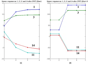
Figure 2-8. Flow diagram of the experimental procedure

Sensors' outputs

Signal preprocessing

Wavelet decomposition

Dimensionality reduction

Pattern classification

(32)

Table 2-1. Details of the dataset

Dataset no: Odor type No. of classes No. of samples No. of samplings

per sample

1 Bacteria 3 54 60

2 Coffee 5 220 60

3 Soda 10 160 90

Table 2-2. Odor class identity

Class label Bacteria Coffee Soda

1 Salmonella Sulawesy Coke

2 Listeria Kenya Diet Coke

3 E-coil Arabia Pepsi

4 - Sumatra Dr. Pepper

5 - Columbia Cherry Coke

6 - - Cherry Pepsi

7 - - Cheerwine

8 - - RC Cola

9 - - Eckerd Cola

A - - Eckerd Dr. Riffic

(33)

( )

⎥⎥ ⎥ ⎥ ⎥ ⎥ ⎦ ⎤ ⎢ ⎢ ⎢ ⎢ ⎢ ⎢ ⎣ ⎡ k,15 k,2 k,1 k 1,15 1,2 1,1 k 0,15 0,2 0,1 k x x x k t x x x t x x x t 1 Sensor Sensor Sensor 1 0 5 2 1

( )

⎥ ⎥ ⎥ ⎥ ⎥ ⎥ ⎦ ⎤ ⎢ ⎢ ⎢ ⎢ ⎢ ⎢ ⎣ ⎡ m,15 ~ m,2 ~ m,1 ~ 1,15 ~ 1,2 ~ 1,1 ~ 0,15 ~ 0,2 ~ 0,1 ~ x x x x x x 1 x x x 0 5 1 2 1 m T T T Sensor Sensor Sensor (2) 0,1 0,1 ~

where m k

is the response of sensor no. 1 at sampling time = 0.

is the wavelet coefficient of sensor no. 1 at new sampling time = 0.

x

Dimensionality reduction. To determine an appropriate subset, the well known linear feature extractor, Principal Component Analysis (PCA) also know as the Karhunen-Loève expansion, was computed to reduce the dimensionality of the features [1], [7], [8], [10], [20].

Pattern classification. Three methods were used to evaluate the classification accuracy of the compressed features: k- Nearest Neighbor (k-NN), Backpropagation Neural Network (BP-NN), and Radial Basis Function Neural Network (RBF-NN) [17], [18], [19], [20], [21].

Validation. Finally, the classification rates of each classification method were determined by N-fold cross-validation, a technique which is commonly used for comparing

(34)

these methods [7], [9], [21]. Conceptually, the dataset are divided into N subsets. Each time, one of the N subsets is used as the testing dataset and N-1 subsets are used as the training datasets. The classification rate is the average value across N trials of the testing datasets.

2.5 Experimental results

First we applied the first three steps (signal preprocessing, wavelet decomposition, and dimensionality reduction) of the algorithm of Fig. 2-8 to the datasets described in Tables 2-1 and 2-2. One way of presenting the distribution of these features is to create a visual examination of feature projections generated by those three processing steps. Typically, 2-D and 3-D scatter plots are used for this purpose. Scatter plots of the datasets produced are illustrated in Fig. 2-9 to 2-11. These projections are based on the db2 wavelet family with 4-level wavelet decomposition. The results show that each class is well separated from the other classes.

(35)

Figure 2-10. PCA projection of Coffee classes after feature compression based on DWT-

db2-level4

Figure 2-11. PCA projection of Soda classes after feature compression based on DWT-

(36)

Next, the final two steps (pattern classification and validation) of the algorithm of Fig. 2-8 were applied. In each dataset, the classification results from transient feature compressions with three wavelet families (Haar, Biorthogonal1.3, and db2) were compared with the result from the traditional steady-state approach. In addition, we performed three different multilevel wavelet decompositions (3rd-level, 4th-level, and 5th-level) of the db2

wavelet which demonstrate the effects of the different multilevel decompositions on the datasets. The approach for evaluating for each odor classification method is as follows. For the k-NN classifier, trial and error was used to find the number of nearest neighbors (k) which provided the highest classification rate. For the Backpropagation neural network (BP-NN) classifier, a fast learning algorithm based on Levenberg-Marquardt (LM) was applied [6]. The complexities of the BP-NN were measured in terms of the network model by the number of neurons in the input layer and in the hidden layer. For the Radial Basis Function Neural Network (RBF-NN) classifier, the spread factors for the input features were also obtained using trial and error.

For the bacteria dataset, the classification accuracy and complexity of the classifiers are summarized in Table 2-3. Since the number of features obtained from biorthogonal 1.3 and

db2 – 3rd level are greater than the total number of samples, these cases are eliminated from the table. From the remaining cases in Table 2-3, the classification rate of all classifiers from

(37)

Table 2-3. Classification performance results of Bacteria dataset

54 Bacteria samples with 3 classes are evaluated by 5-fold cross validation

k-NN Backpropagation (LM) Radial Basis Function

Type of feature

No. of

features k

% Classification

correct

Network model

% Classification

correct

Spread factor

% Classification

correct

Stead-state 4 3 98.14 4-3 93.47 1 87.03

Haar-3rd

level 5 5 80.40 2-3 83.80 3 78.00

Db2-4th

-level 5 3 100 2-3 99.60 3 98.00

Db2-5th

level 3 3 100 2-3 99.20 3 98.00

(38)

Table 2-4. Classification performance results of Coffee dataset

220 coffee samples with 5 classes are evaluated by 5-fold cross validation

Type of feature

No. of

features k

% Classification

correct

Network model

% Classification

correct

Spread factor

% Classification

correct

Stead-state 4 3 55.45 4-8-5 57.27 0.4 60.45

Haar-3rd

level 5 3 68.95 3-4-5 77.00 1 88.60

Bior1.3-10th level

5 3 85.45 3-4-5 97.54 3 91.81

Db2-3rd

level 6 3 78.86 3-4-5 94.36 3 92.27

Db2-4th

-level 6 3 84.81 3-4-5 94.59 3 95.45

Db2-5th

level 4 3 96.31 3-4-5 95.45 3 96.36

(39)

Table 2-5. Classification performance results of Soda dataset

160 coffee samples with 10 classes are evaluated by 5-fold cross validation

Type of feature

No. of

features k

% Classification

correct

Network model

% Classification

correct

Spread factor

% Classification

correct

Stead-state 4 3 55.50 4-9-10 75.00 2 70.00

Haar-3rd

level 5 3 55.68 4-8-10 54.18 3 52.50

Bior1.3-10th level

5 3 91.75 4-8-10 83.68 3 93.75

Db2-3rd

level 6 3 91.12 4-8-10 82.50 3 89.37

Db2-4th

-level 6 3 96.56 4-8-10 84.06 3 95.00

Db2-5th

level 6 3 97.43 4-8-10 86.50 3 95.62

2.6 Discussion

(40)

extraction. Supporting this hypothesis, as expected, transient feature compressions in our study using Daubechies and Biorthoginal wavelets provide better classification performance than does the Haar wavelet.

2.7 Conclusions

Perhaps the most challenging specifications for designers of machine olfaction instruments are classification accuracy and the classification speed, especially in high dimensional input spaces generated by large odor sensing arrays. Typically, a complex classifier is designed for the high dimensional input feature space that leads to a time-consuming computationally limited implementation with substandard classification accuracy. Front-end processing to extract a reduced set of input features is required. From our experimental results, transient feature compression based on DWT provides a satisfactory tool in terms of not only improving all above issues but also reducing the data acquisition time and prolonging the sensor’s lifetime.

2.8 References

[1] B. G. Kermani, On using neural networks and genetic algorithms to optimize the performance of an electronic nose, Ph.D. dissertation, North Carolina State Univ., Raleigh, 1996.

[2] R. Gutierrez-Osuna, Signal processing and pattern recognition for an electronic nose, Ph.D. dissertation, North Carolina State Univ., Raleigh, 1998.

(41)

[4] K. Arshak, E. Moore, G.M. Lyons, F. Harris, and S. Clifford, A review of gas sensors employed in electronic nose application, Sensor Review, vol. 24, no. 2, 2004, pp. 181-198.

[5] R. Gutierrez-Osuna and H. T. Nagle, A method for evaluating data-preprocesing techniques for odor classification with an array of gas sensors, IEEE Trans Syst. Man Cybern. B, vol. 29, pp. 626-632, May 1999.

[6] R. Gutierrez-Osuna, H. T. Nagle, B. Kermani, and S. Schiffman, Signal conditioning and preprocessing, in Handbook of Machine Olfaction: Electronic Nose Technology, T. C. Pearce, S. S. Schiffman, H. T. Nagle, and J. W. Gardner, Eds. Weinheim, Germany: Wiley-VCH, 2002.

[7] K. Jain, R. P.W. Duin, and J. Mao, Statistical pattern recognition: a review, IEEE Transactions on Pattern Analysis and Machine Intelligence, vol. 22, no. 1, pp. 4-37, 2000.

[8] M. Pardo and G. Sberveglieri, Learning from data: a tutorial with emphasis on modern pattern recognition methods”, IEEE Sens., vol. 2, no. 3, pp. 203-217, 2002.

[9] R. Gutierrez-Osuna, Pattern analysis for machine olfaction: a review, IEEE Sens., vol. 2, no. 3, pp. 189-202, 2002.

[10] V. Cherkassky and F. Mulier, Learning from data: concepts, theory, and methods, New York, Wiley, 1998.

(42)

[12] C. Distante, M. Leo, P. Siciliano, and K. C. Persaud, On the study of feature extraction methods for an electronic nose, Sens. Actuators B, vol. 87, pp.274-288, 2002.

[13] L. M. Bruce, C. H. Koger, and J. Li, Dimensionality reduction of hyperspectral data using discrete wavelet transform feature extraction, IEEE Trans., Geoscience and Remote Sensing, vol. 40, no. 10, pp. 2331-2338, 2002.

[14] L. A. Klein, Sensor and data fusion concepts and applications, 2nd ed. Bellingham, WA: SPIE, 1999.

[15] R. Gutierrez-Osuna, H. T. Nagle, and S. Schiffman, Transient response analysis of an electronic nose using multi-exponential models, Sens. Actuators B, vol. 61, no. 1-3, pp.170-182, 1999.

[16] M.L. Rodriguez-Mendez, A. A. Arrieta, V. Parra, A. Bernal, A. Vegau, S. Villanueva, R. Gutierrez-Osuna, J. A. de Saja, Fusion of three sensory modalities for the multimodal characterization of red wines, IEEE Sens., vol. 4, no. 3, pp. 348-354, 2004.

[17] C. M. Bishop, Neural network for pattern recognition, New York: Oxford Univ., 1995.

[18] H. Demuth and M. Beale, Neural network toolbox user’s guide: for use with matlab, ver. 4, MA, MathWorks, 2004.

(43)

[20] R. O. Duda, P. E. Hart, and D. G. Stork, Pattern classification, 2nd ed. New York: Wiley, 2000.

(44)

Chapter 3 Sensor selection for electronic noses based on wavelet transient

feature extraction

3.1 Abstract

Machine olfaction devices, often called electronic noses, are gaining favor for odor assessment applications in several industrial sectors such as beverage, perfumery, and food. From a design point of view, the number of sensors in these devices for a particular application should be minimized without degrading classification accuracy. This chapter deals with selecting sensors for electronic noses in order to make possible small portable devices with fast response times and reduced cost. Prior research efforts have reported in the open literature have applied data mining methods to feature subset selection and have shown that many advantages can be gained by properly selecting the input feature before forwarding to a pattern classification algorithm: reduce the dimensionality of the feature space, remove redundant and irrelevant features, speed up a classification process, and improve a classification performance. In this study, the data mining feature subset selection process is adapted to tailor a gas sensor array for three different odor sample sets (bacteria, coffee, and soda). From experimental results, the output features obtained by applying a Discrete Wavelet Transform (DWT) to the transient sensor responses not only provide a significant reduction in the number of sensors when compared to traditional features, but also improve the classification rate to near 100 %.

(45)

3.2 Introduction

Typically, an electronic nose consists of three functional components that sequentially operate as shown in Fig. 3-1. The sampling unit contains an array of sensors with broad sensitivities that provide dynamic responses of the interaction between an odor sample and the sensing elements [1]. A fundamental design concept for an array of sensors used in the electronic nose is that each sensor should have a different sensitivity profile over the range of compounds expected in the target application. Therefore, the array of sensors provides distinct response patterns to different odors.

The next element on Fig. 3-1 is the signal-processing function. Signal processing is applied for several purposes. Generally, the responses from the array of sensors are affected by several interfering environment factors such as varying operating temperature and changing relative humidity that give unstable responses over time [2]. Signal processing can compensate for these conditions [3]. In addition, reducing the dimensionality of the sensor feature space and extracting informative sensor features are also performed by the signal-processing block.

(46)

Figure 3-1. Typical block diagram of an electronic nose

Researchers have proposed many algorithms to choose a near-optimal subset of the original features; this process is called feature subset selection (FSS) [5], [6], [7]. In practice, some or most of the sensor features are redundant and irrelevant depending on the sensor sensitivities and odor characteristics. Thus, odor classification, in general, requires a complex algorithm that can lead to poor generalization and time-consuming execution. Ideally, highly informative and uncorrelated features can be found. Some researchers have reported impressive results after applying feature subset selection in particular applications [8], [9]. In addition to reducing the dimensionality of the feature space, high prediction performance was successfully obtained. In this study, we show that the features from multilevel decomposition based on the discrete wavelet transform (DWT) provide a significant sensor reduction and also a classification rate that is near perfect.

The organization of this study is as follows. In section 3.3, we will describe the principles of the transient feature extraction from DWT. Section 3.4 reviews a feature subset selection applied to select sensors in the array. Details of the search algorithms applied in our study are given in section 3.5. Section 3.6, we explain an experimental details and results of the study are shown in section 3.7. Discussion and conclusion are drawn in section 3.8 and 3.9, respectively.

Odor Sample

Sampling Unit

Signal Processing

Odor Classification

(47)

3.3 Transient feature extraction based on wavelet decomposition

A brief overview of wavelet analysis applied to this study is described first. A more detail of wavelet can be found in appendix. In general, a signal or function f t

( )

from a space

S can be represented as a linear combination as shown in (1).

( )

_i _i (1)

i

f t =

∑

α ϕ

where is an expansion coefficient.

is a set of functions of or an expansion set. is an integer index of a finite or infinite number i i t i α ϕ ∈ Z

In DWT analysis, a wavelet system is created by simply scaling (j) and translating (k) a single scaling function or a single wavelet function as shown in (2) and (3). In general, a function ψ (t) is called a mother wavelet. The goal is to generate a set of basis function such that any signal or function f t

( )

∈L2can be expressed by linear combination of the scaling and wavelet functions as shown in (7).

( )

(

)

( )

(

)

( )

2

2 2 2

2 2 3

j/ j j,k

t t k

ψ t ψ t k

ϕ = ϕ − = −

( )

0 0 0 , , , , (4) , (5) 6

j k j k j k

j j ,k j j,k

k k j j

f t a t

f t t t

a k t d k ψ t

(48)

( )

(

)

( )

(

)

( )

0 0 0 0 2 2

2 2 2 2 7

where is called scaling coefficients. is called wavelet coefficients.

( integer number )

j / j j/ j

j j

k k j j

j j

a k t k d k ψ t k

a k d k

j , k , n

ϕ ∞

=

= − + −

∈

∑

∑ ∑

The advantages of wavelet representation over other expansion approaches include a time-frequency localization property and a multiresolution property. For time-frequency localization, the DWT can provide time and frequency parameters for specific dynamic signal events. Regarding multiresolution property, the scaling and wavelet basis functions can be scaled and translated depending on the j and k parameters as shown in (2) and (3). As a result, the original signal can be represented by different scaled and translated wavelet basis functions as shown in (7). The wavelet functions can be adjusted and a large number of wavelet basis functions can be designed for a particular application [10], [11]. In general, wavelet analysis is most suitable for transient signals whose statistical characteristics vary over time, whereas Fourier analysis is appropriated for periodic signals.

( )

[

]

( )

[

]

( )

0 1

1 1

Solving for and in (7)

2 8 2 9 where 2 j j j j m j j m

a k d k ,

a k h m k a m

d k h m k a m

m k n

+ + = − = − = +

∑

The classical method of computing the discrete wavelet transform can be implemented by a two-channel filter bank which is pioneered by S. Mallat [12] shown in Fig. 3-2(a). The filter bank consists of h n₀[- ] coefficients or lowpass filter (LPF) and h n₁[- ] coefficients or

(49)

bank. In general, the low frequency component represents the identity of the original signal [13]. By discarding the high frequency component and forwarding the low frequency component sequentially to the next filter bank as shown in Fig. 3-2 (b), the original signal can be decomposed to a multilevel approximation. Hence, the original signal can be approximated by the multilevel decomposition of the signal at various levels of resolution.

Figure 3-2. (a) A two-channel filter bank, (b) Mulitlevel two-channel filter banks

An example of two-level signal decomposition applied to a sensor’s response is illustrated in Fig. 3-3. At point 1, a sensor’s dynamic response is applied to the first filter bank. At point 2, the output of the lowpass filteris displayed. Note that a lowpass filter can consider conceptually to perform a neighborhood average between sampling points. At point 3, the output of the lowpass filter is downsampled by a factor of 2; only even samples are kept. At point 4, the output of the lowpass filter of the first filter bank is forwarded to the

aj

aj+1 2

2 dj

(a)

LPF h0[-n]

HPF h1[-n]

2

aj+1 ₂ aj

dj 2

2 aj-1

dj-1 (b)

LPF h0[-n]

HPF h1[-n]

LPF h0[-n]

(50)

lowpass filter of the second filter bank. Note that the output of the second filter bank is smoother than that of the first filter bank. At point 5, the downsampling output from the second filter bank is illustrated. Note that after discarding the high frequency components, the general shape of the final output is similar to that of the original signal. Hence, the input signal can be approximated by multi-level low frequency components. From the multi-level decomposition point of view, we can say that the output signal from the lowpass filter is an average version of the input signal but it can be represented by smaller number of sampled points.

Figure 3-3. Example of 2-level signal decomposition for two-channel filter banks

aj

aj+1 _LPF ₂

HPF 2 dj

LPF 2 aj-1

HPF 2 dj-1

0 1 2 3 4 5 6 7 8 9 10 11 12 13 14

1

(51)

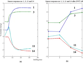
As shown above, the important benefit of the multilevel decomposition in signal representation is that we can reduce the number of sampling points of the signal while keeping the original signal’s general characteristics. This concept applied in this study for sensor’s responses to a given odor is the same as an approach we use to extract transient features in chapter 2. As an example, the responses from sensors no. 1, 3, 11 and 14 of a given coffee exposure are plotted in Fig. 3-4(a) which consists of 32 sampling points for each sensor. In Fig. 3-4(b), only 4 sampling points for each sensor are obtained from a 4th-level decomposition based on db2-wavelet to represent the original sensor responses. These features from multilevel decomposition will be investigated to optimize the number of sensors using in an electronic nose device.

Figure 3-4. (a) Example of sensor responses of a particular coffee class, (b) 4th-DWT of sensor responses based on “db2”[11].

1 3

11 14

1

3

11

(52)

3.4 Feature Subset Selection

The main reasons to reduce the dimensionality of a feature space are classification accuracy and measurement cost [15], [16]. For classification accuracy, dimensionality reduction would be simplified if different sample types were clearly distinguished from other sample classes. However, the sensors in the array are likely to have cross-sensitivity. Consequently, sensors should be chosen to 1) maximize the overall sensitivity and selectivity of the array, 2) maximize the classification performance of the system, and 3) minimize the execution time of the classification process [8]. In addition, a wise choice of sensors to be included in the array can mitigate the curse of dimensionality that occurs when a limited number of application-specific odor samples are available for training the electronic nose [17].

For dimensionality reduction of features, there are two terms that are used to describe the process: feature extraction and feature subset selection. Feature extraction is based on methods that create new features by manipulating on the original features (y f x= ( ) : d → mwherem d< ). Feature subset selection refers to algorithms which choose a feature subset of size m from the original feature set of size d, where m < d [15]. In this work, we use multilevel decomposition of the sensors’ transient responses as our feature extractor, then apply feature subset selection to choose the best sensor subset.

(53)

Figure 3-5. Flowchart of general procedure of feature subset selection

The first step, subset generation, is regarded as the most important since it functions to generate candidate subsets that improve e-nose performance. Basically, it is a search procedure to provide candidate subsets for evaluation. The most straightforward method is to examine all possible combinations of the original features (2d combinations), often called

exhaustive search. Although, this approach is guaranteed to find the optimal feature subsets, the total number of possible subsets is impractical for computation even for a moderate number of original features d [6]. Therefore, the problem of feature subset selection is crucial for implementing a practical solution. After feature subsets are generated, in the second step each feature within the subset is evaluated by an objective function and is compared to the previously identified best feature. If a better feature is found, the previous best feature will be replaced. In each pass through the algorithm, a subset of features selected for evaluation is called the current generation. The stopping criteria are checked in the third step to determine if computation should continue. The basic stopping rules used herein are 1) a predefined

Subset generation

Subset evaluation

Stopping criterion

Subset validation

Selectedfeatures(m)

Originalfeatures (d)

Yes

(54)

number of subset features are found, 2) a predefined number of generations are reached, 3) a target value of the objective function is met, or 4) the value of the objective function has no improvement over a predetermined number of generations. Finally in the fourth step, selected feature subsets must be validated using unseen samples.

At this point, we can see that the search method is a key in the feature subset selection. We have to decide the starting point for each search, what the directions to search, and how to search (the search techniques). In practice, search methods can be classified in three ways: complete, heuristic, and random. Complete search is a simple method and means that every possible feature subset must be evaluated; it is exhaustive. This method is infeasible for even a moderate number of features due to its computational requirements. Hence, we might accept suboptimal performance in a trade for computational efficiency.

Heuristic search seeks to improve performance by truncating a complete search using special techniques such as Branch and Bound [18]. This method can find the optimal feature subsets without exhaustive search, but the objective function to be evaluated must satisfy the monotonic principle. Unfortunately, the objective function, classification rate, used to evaluate sensors for an e-nose doesn’t comply with this principle. So, this algorithm cannot be applied in this study.

(55)

because it is known that optimal larger feature subsets do not necessarily contain optimal smaller feature subsets [19].

Unlike the sequential strategies in which the features grow or shrink at each generation, the random search method performs a global search from a current population of possible solutions and improves the quality of a population with each pass through the algorithm. This strategy is basically inspired by a process of natural selection as has been employed in the past such methods as the genetic algorithm (GA) and simulated annealing (SA). The advantage of this approach is that most of the time it can find the optimal solution with smaller numbers of combinations than 2d [9].

(56)

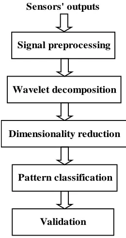
Our goal in this study is to maximize the classification rate of an e-nose with the least number of sensors. Hence, our application is very dependent on the selected learning algorithm and the wrapper method will be used for feature evaluation in the sensor selection algorithm of Fig. 3-5.

Figure 3-6. Block diagrams of filter feature subset selection (FSS) and wrapper FSS methods

3.5 Details of the search algorithms

In this study, we will investigate the effectiveness of wavelet transient feature extraction for e-nose sensor selection and compare the results to previous work performed by Gutierrez-Osuna [14] in terms of the optimal number of sensors using in an electronic nose and classification accuracy. In his study, Gutierrez-Osuna employed bell-shaped windowing

Input features

ML algorithm Search algorithm

Feature evaluation Filter FSS

Data characteristic Feature

subset

Selected features

Input features

ML algorithm

Selected features Search algorithm

Wrapper FSS

Predictive accuracy Feature

subset

(57)

functions rather than wavelets to segment a sensor’s transient response. In this study, two search strategies based on the wrapper method were applied after wavelet transient feature compression to minimize the number of sensors in an array for an electronic nose machine: sequential search and random search.

Sequential search method: To reduce massive amount of computation required for an exhaustive search, heuristic search strategies have been proposed to implement computational efficiency [21]. The widely used sequential greedy search method appears to provide a computational advantage but, in general, yields a suboptimal solution. Using such strategies doesn’t always mean that one must sacrifice classifier performance. It turns out that in some cases near-optimal results can be obtained [22]. Herein, we use sequential forward sensor subset selection and sequential backward sensor subset selection as displayed in Fig. 3-7 and 3-8, respectively.

Figure 3-7. A procedure of sequential forward sensor subset selection 0. Set a target classification rate.

1. Start with an empty set of "selected" sensors.

2. One at a time, insert each of the remaining unselected sensors into the "selected" set and calculate the classification rate.

3. Sort the unselected sensors by their effect on the classification rate.

4. Choose a single sensor providing the highest classification rate improvement and transfer it into the "selected" set.

(58)

Figure 3-8. A procedure of a sequential backward sensor subset selection

Random search method: Although sequential search provides a computational advantage, some sequential search algorithms trend to get trapped in local solutions. To avoid these local entrapments, a random search method has been proposed to provide a global solution while limiting computational demands. One of the most effective and widely used random methods is the genetic algorithm (GA) which is inspired from biological evolution [23]. Conceptually, the GA repeatedly modifies parent population sets of possible solutions by using three main strategies to generate new children population sets [24]. These are selection rules, crossover rules, and mutation rules. The selection rules are employed to choose members of current individual populations to establish a next generation of elite children. Elite children are copied from the current population set based on a predefined “fitness” metric. The crossover rules elaborate ways to combine two individual populations for a next generation containing crossover children. Crossover children can be selected by several methods (e.g., by fitness or randomly). The mutation rules make random changes to individual member in a given population to create a next generation of mutation children.

0. Set a target classification rate.

1. Start with a set containing all of the sensors.

2. Compute the classification rate ignoring one sensor at a time. 3. Sort the sensors their effect on the classification rate. 4. Discard the sensor having the least contribution.

(59)

Figure 3-9. A procedure of the Genetic algorithm (GA)

The GA procedure being applied for sensor selection is shown in Fig. 3-9. The classification rate, the function that we want to maximize, is chosen as the fitness function that measures the goodness of each sensor population. In this algorithm, the sensor selection problem is encoded as an n-binary vector in which each entry in the vector represents an ith sensor in the array. A 0 or 1 is used to indicate an absence or present of a specific sensor. A pictorial operation of the GA for sensor subset selection is shown in Fig. 3-10. At step 1, an initial population of m sensor subsets is randomly generated from n total sensors (n = 15 in our case). This creates the initial generation. In the next step, each individual sensor subset is evaluated by the fitness function (classification rate). In this case, a k-nearest neighbor (k-NN) is applied to compute the classification rate. Then, the stopping criteria, which are based on the target fitness values from each population and the maximum number of allowed generations, are checked. A 100% classification rate and 20 generations are used in this experiment for stopping criteria. So, the GA will be stopped whenever either those conditions are met. If the stopping criteria fail, the GA modifies the current generation of sensor subset sets by using selection rules, crossover rules, and mutation rules. In Fig. 3-10, we illustrate the operation of the procedure. First, m sensor subsets are created by some predefined method (randomly, by sensor cost, or by some other application-specific constraints). Next the population of m sensors subsets is evaluated. For our example, assume that sensor subsets

0. Set a target stopping value (classification rate and number of generations). 1. Generate a random initial population (generation) of sensor subsets. 2. Evaluate the fitness of each sensor subset and check the stopping criteria. 3. Rank the fitness scores of each subset.

4. Choose two parent subsets based on their fitness scores.

5. Produce a new population (generation) from the parents by operating crossover and mutation.

(60)

(61)

1. Create initial population S ensor no: 1 S ensor no: 2 S ensor no: 3 S ensor no: 4 S ensor no: 5 S ensor no: 6 S ensor no: 7 S ensor no: 8 S ensor no: 9 S ensor no: 10 S ensor no: 11 S ensor no: 12 S ensor no: 13 S ensor no: 14 S ensor no: 15

Sensor subset no: 1 1 1 0 0 1 0 0 1 0 0 0 1 0 0 1

Sensor subset no: 2 0 1 1 0 0 0 1 1 0 0 1 0 0 0 0

Sensor subset no: m 0 0 1 0 0 1 1 0 0 0 0 0 0 1 0

2. Evaluate each sensor subset and check stopping criteria

3. Produce new population

- Select good population

Sensor subset no: 1 1 1 0 0 1 0 0 1 0 0 0 1 0 0 1

Sensor subset no: 2 0 1 1 0 0 0 1 1 0 0 1 0 0 0 0

- Perform crossover

Sensor subset no: 1 1 1 0 0 1 0 0 1 0 0 1 0 0 0 0

Sensor subset no: 2 0 1 1 0 0 0 1 1 0 0 0 1 0 0 1

- Perform mutation

Sensor subset no: 1 1 1 0 1 1 0 0 1 0 0 1 0 0 0 0

Sensor subset no: 2 0 1 1 0 0 0 0 1 0 0 0 1 0 0 1

Crossover point

Classification algorithm

Signal Processing using Wavelets for Enhancing Electronic Nose Performance

Abstract

SIGNAL PROCESSING USING WAVELETS FOR ENHANCING

ELECTRONIC NOSE PERFORMANCE

EKACHAI PHAISANGITTISAGUL

ELECTRICAL ENGINEERING

APPROVED BY:

Biography

Acknowledgements

Table of Contents

List of Tables

List of Figures

Chapter 1

Introduction

1.1

Overview

1.2

The history of the electronic nose

1.3

Why an electronic nose

1.4

Purpose of this research

1.5

Organization of this dissertation

1.6

References

Chapter 2

Transient feature extraction based on wavelet decomposition for

pattern classification of electronic noses

2.1 Abstract

2.2

Introduction

2.3

Transient feature extraction based on wavelet decomposition

2.4

Experimental procedures

( )

( )

( )

( )

( )

( )

( )

( )

( )

( )

2.5

Experimental results

2.6

Discussion

2.7

Conclusions

2.8

References

Chapter 3

Sensor selection for electronic noses based on wavelet transient

feature extraction

3.1 Abstract

3.2

Introduction

3.3

Transient feature extraction based on wavelet decomposition

( )

( )

∑

( )

( )

(

)

( )

( )

(

)

( )

( )

( )

( )

( )

( )

( )