Resilient Reliable Dynamic-output-feedback Control for Takagi-Sugeno Fuzzy Time-Delayed Systems with Time-Varying Actuator Fault

Resilient Reliable Dynamic-output-feedback Control

for Takagi-Sugeno Fuzzy Time-Delayed Systems

with Time-Varying Actuator Fault

S. Senpagam1, P. Dhanalakshmi2, R. Mohana Priya3

Department of Applied Mathematics1,2,3_{, Bharathiar University, Coimbatore 641 046, India.}

Email:[email protected]_{, [email protected],[email protected]}

Abstract—This article investigates the reliable dynamic-output-feedback problem for a class of Takagi-Sugeno (T-S)

fuzzy model subject to time-varying delay and actuator fault. The main intention is to design a fault-detection mixed H∞ and passivity based dynamic-output-feedback controller that guarantees the resulting closed-loop system

to be asymptotically stable by using adaptive fault estimation algorithm subject to admissible time-varying actuator faults. More precisely, the asymptotic stability of the concerned system is obtained by constructing an appropriate Lyapunov-Krasovskii functional and novel sufficient stabilization conditions in terms of linear matrix inequalities are established with a prescribed disturbance attenuation level. Finally, the simulation studies are incorporated to exhibit the power of prescribed control design.

Keywords: T-S Fuzzy systems, Time-varying actuator failure, Fault estimation, Dynamic-output-feedback.

1. Introduction

In recent years, fuzzy dynamical systems in the texture of Takagi-Sugeno (T-S) model have rapid growth due to its attractive features [1]- [5]. Moreover many real-world systems exhibit nonlinear characteristics which bring severe difficulties during the process of stabilization. T-S fuzzy model based approach provides an efficient way to analyse and synthesize nonlinear systems [6]-[8]. On the other hand, T-S fuzzy model with time-delay cause nonlinear retarded systems. Therefore the issue of time-delay has been taken into account in T-S fuzzy model by many researchers. By constructing a novel augmented Lyapunov-Krasovskii(L-K) functional, Kwon et al. in [9] designed stability conditions for T-S fuzzy systems with time-varying delay. In [10] the problem of delay-dependent stability is discussed for T-S fuzzy systems with time-varying delay.

Obviously, many engineering systems in the real world cannot work perfectly at all times under all situations. In order to acquire higher safety and reliability criterion, the possible faults which may affect the system performance have be able to detected and

identified as early as possible. To estimate such faults, observer-based fault detection, isolation and fault tolerant control using T-S fuzzy model have gained considerable interest [11]. Youssef et.al [13] designed a Proportional Integral observer for estimating the actuator and sensor faults with unmeasurable premise variables based on T-S fuzzy model. A novel fault estimation and fault tolerant control has been proposed in [14] for T-S fuzzy sytems with time-varying state delay against actuator faults. In particular, some practical systems may have time varying faults. The fault detection technique is employed to handle these kinds of time-varying faults. With the aid of Kalman-Yakubovic-Popov lemma in a local linear model, fault detection filter system and the dynamics of filtering error generator are constructed in [15] for T-S fuzzy discrete systems. The fault detection problem for continuous-time T-S fuzzy systems in finite frequency domain against sensor faults is studied in [16]. The problem of fault detection, isolation and estimation of nonlinear systems using T-S fuzzy model is proposed in [17], wherein the minimization problem

is formulated by bounded real lemma and Polya’s theorem is used to reduce the conservatism.

In many real-world systems, state-feedback control appraoch will fail to guarantee the stabilizability when complete knowledge of the system is not known. In such cases, observer-based dynamic output feedback control is need to be designed so that the unmeasurable states can be estimated from the dynamical process. Moreover, the observer-based dynamic feedback control plays a positive role in system performance and stabilizing the unstable systems. Therefore, this control using T-S fuzzy model approach for dynamical systems has attracted remarkable attention in the control theory ( [18]- [19]). By employing the reciprocally converse approach, in [20] an investigation is made on dynamic-output-feedback control for T-S fuzzy system with time-varying input delay and output constraints. The robust dynamic output feedback control problem for a class of discrete-time nonlinear systems is investigated in [21], by employing T-S fuzzy model. External noises are common barrier for the process of stabilization of dynamical system-s, which should be controlled or removed by using some performance. The local H∞ control problem is

designed in [22] for the continuous-time T-S systems where the derived LMIs are solved by means of Convex Optimization Technique. A novel robust H∞ dynamic

sliding mode control is proposed in [24] for a class of uncertain stochastic nonlinear systems, wherein a new set of conditions guaranteeing the stochastic stability are derived in terms of LMIs. The problem of mixed H∞ and passivity performance analysis and design is

discussed in [23] for discrete time-delay neural networks represented by T-S fuzzy model. Yet, to the authors best knowledge, the fault estimation control together with the dynamic-output-feedback and mixed H∞ and passivity

performance has not been studied for T-S fuzzy systems. Motivated by this thought, this investigation deals on the stabilization of the T-S fuzzy time-delayed system with the incorporation of fault-tolerant dynamic-output-feedback control via adaptive fault estimation algorithm. 2.Problem formulation and preliminaries

In this section our focus is to construct the closed-loop system by using dynamic-output-feedback control.

Consider the following T-S fuzzy model with time-varying delay:

System rule p: If g1(x(t)) is M1p and g2(x(t)) is Mp2 and . . . and gp(x(t))is Mp_h then

˙

x(t) =Apx(t) +Adpx(t−τ(t)) +Bpu(t) +Dpω(t) +Bapf(t),

y(t) =Cx(t), (1)

where p ∈ {1,2, . . . , l}, l is the number of T-S fuzzy system rules,gq(x(t))are premises variables andMpqare

fuzzy sets. Letx(t) = [xT₁ xT₂ . . . xT_n]T be state vector, y(t)is the output signal,τ(t)denotes time-varying delay with τ1 ≤ τ(t) ≤ τ2 < ∞ for some τ1 ≥ 0 and τ2 >0, u(t) andω(t) stands for control input and time-varying actuator fault respectively, f(t) denotes noice term andAp,Adp,Bp,BapC,Dp are system parameters

of appropriate dimensions. Then the over all T-S fuzzy model based on (1) can be written in the form,

˙

x(t) = l

X

p=1

ϕp(g(t)){Apx(t) +Adpx(t−τ(t)) +Bpu(t)

+Dpω(t) +Bapf(t)}, (2)

y(t) =Cx(t), (3)

where ϕp(gp(x(t))) = $p(gp(x(t))) l

P

p=1

$p(gp(x(t)))

,

$p(gp(x(t))) = Πhq=1M

p

q(gp(x(t))) , g(t) = [g₁T(x(t)) gT₂(x(t)). . . g_hT(x(t))]T and Mpq(gq(x(t)))

represents membership degree of gp(x(t)) in Mpq. Let

A(ϕ) = l

P

p=1

ϕp(g(t))Ap, Ad(ϕ) = l

P

p=1

ϕp(g(t))Adp,

B(ϕ) = l

P

p=1

ϕp(g(t))Bp, Ba(ϕ) = l

P

p=1

ϕp(g(t))Bap and

D(ϕ) = l

P

p=1

ϕp(g(t))Dp. Then the system (2) can be

rewritten in the following form:

˙

x(t) =A(ϕ)x(t) +Ad(ϕ)x(t−τ(t)) +B(ϕ)u(t) (4) +D(ϕ)ω(t) +Ba(ϕ)f(t),

y(t) =Cx(t). (5)

Taking the effects of actuator fault into account and by implementing adaptive algorithm, the fuzzy observer is constructed in the following form to estimate the faults:

Observer rule p: If g1(xO(t))is Mp₁ and g2(xO(t)) is Mp₂ and . . . and gp(xO(t)) is Mp_h then,

˙

xO(t) =ApxO(t) +AdpxO(t−τ(t)) +Bpu(t) +BapfO(t) +Lp[yO(t)−y(t)], (6)

yO(t) =CxO(t), (7) ˙

fO(t) =−P4−1Fp[ ˙ey(t) +ey(t)], (8)

where xO(t) denotes observer state, fO(t) is estimated

fault and Lp represents observer gain to be determined.

After the process of de-fuzzyfication as discussed above the observer system becomes,

˙

xO(t) =A(ϕ)xO(t) +Ad(ϕ)xO(t−τ(t)) +B(ϕ)u(t) +Ba(ϕ)fO(t) +L(ϕ)[yO(t)−y(t)], (9)

yO(t) =CxO(t), (10) ˙

fO(t) =−P₄−1F(ϕ)[ ˙ey(t) +ey(t)], (11)

where Lp and Fp are the unknown gains, P4−1 repre-sents learning rate, L(ϕ) =

l

P

p=1

ϕp(g(t))Lp, F(ϕ) =

l

P

p=1

ϕp(g(t))Fp, and ey(t) = yO(t)−y(t). Let e(t) =

xO(t)−x(t), then the error system can be expressed in

the following form:

˙

e(t) =[A(ϕ) +L(ϕ)C]e(t) +Ad(ϕ)e(t−τ(t)) −D(ϕ)ω(t) +Ba(ϕ)ef(t) (12)

ey(t) =Ce(t), (13)

where ef(t) =fO(t)−f(t).

In order to design a controller in a more effective and unbreakable way, a resilient reliable dynamic-output-feedback fuzzy controller is designed in the following form,

Controller rule p: If g1(xc(t)) is Mp1 and g2(xc(t)) is Mp₂ and . . . and gp(xc(t))is Mph then,

˙

xc(t) =Acpxc(t) +Bcpy(t), (14)

u(t) = (Kp+δK(t))xc(t)−B+(ϕ)Ba(ϕ)fO(t),

(15)

where Ac, Bc, Kq are controller gains, B+(ϕ) = BT_(ϕ)

BT_(ϕ)B(ϕ) and δK(t) represents the gain fluctuation

which is described in the form δK(t) = MKF(t)NK

whereMK,NKare known suitable dimensional matrices

withFT_{(t)F(t)≤I is Lebesgue measurable. Moreover,}

by the de-fuzzification process the following equations can be obtained,

˙

xc(t) =Ac(ϕ)xc(t) +Bc(ϕ)y(t), (16)

u(t) = (K(ϕ) +δK(t))xc(t)−B+(ϕ)Ba(ϕ)fO(t),

(17)

where Ac(ϕ) = l

P

p=1

ϕp(g(t))Acp, Bc(ϕ) =

l

P

p=1

ϕp(g(t))Bcp and K(ϕ) = l

P

q=1

ϕq(g(t))Kq. By

substituting (17) into (5), the closed-loop is obtained in the following form,

˙

x(t) =A(ϕ)x(t) +Ad(ϕ)x(t−τ(t)) +B(ϕ)(K(ϕ) +δK(t))xc(t) +D(ϕ)ω(t)−Ba(ϕ)ef(t),

(18)

y(t) =Cx(t). (19)

By defining the augmented vector η(t) as

[xT(t) eT(t) x_cT(t) eT_f(t)]T and combining the equations (11) - (19) the augmented form of T-S fuzzy system can be written as,

˙

η(t) =Aη(t) +Adη(t−τ(t)) +Dω(t) +Baf˙(t),

(20)

A =



  

A(ϕ) 0 A13 −Ba(ϕ)

0 (A(ϕ) +L(ϕ)C) 0 Ba(ϕ)

Bc(ϕ)C 0 Ac(ϕ) 0

0 A42 0 A44



   ,

A13 = B(ϕ)(K(ϕ) + δK(t)), A42 =

−P₄−1F(ϕ)C[A(ϕ) +L(ϕ)C+ 1], A44 = −P4−1 F(ϕ)CBa(ϕ),

Ad =



   

Ad(ϕ) 0 0 0

0 Aa(ϕ) 0 0

0 0 0 0

0 −P₄−1F(ϕ)CAd(ϕ) 0 0



    ,

D=



   

D(ϕ) −D(ϕ)

0

P₄−1F(ϕ)CD(ϕ)



   

andBa=



   

0 0 0 −1



    .

In order to derive the required theoretical result, consider the following assumptions, definition and lemmas:

Assumption 1. f˙(t) is norm bounded. i.e. ||f˙(t)|| ≤

fmax where0≤fmax<∞.

Assumption 2. Rank(CBap) = r, wherer is the rank

of Bap.

Assumption 3. Invariant zeros of (Ap, Bap, C) lie in

open left plane.

2.1. Lemma [12]Let the Assumption 2 and Assumption 3 hold then there exist a positive definite matrixP2 such that the following condition holds, F(ϕ)C =B_aT(ϕ)P2.

2.2. Lemma [21] Let matrices X, Y and Z(t) be real matrices with appropriate dimensions and Z(t)

satisfying ZT(t)Z(t) ≤ I is lebeque measurable, then for any scalar > 0, the following inequality holds, XZ(t)Y +YTZ(t)XT ≤XXT +−1YTY.

2.3. Definition [23] For given positive scalar γ and θ ∈ [0,1], the constructed T-S fuzzy system (19) achieves asymptotic stability with

the performance mixed H∞ and passivity iff

γθ−1yT(t)y(t)−2(1−θ)yT(t)ω(t)−γωT(t)ω(t) ≤0

where,θ=

 



1 if H∞

0 if P assivity.

3. Main results

This section deals with the stability analysis of the prescribed system by employing L-K functional and adaptive algorithm. In order to do this, it is sufficient to prove that the system (5) is asymptotically stable with the prescribed performance index. To be precise, the following theorem presents the sufficient conditions guaranteeing the asymptotic stability of the system (5) without considering the gain fluctuations. From these conditions, the dynamic-output feedback controller is obtained in Theorem (2) by considering gain fluctuations. 3.1. Theorem Let the Assumptions 1-3 hold. For given

positive scalars γ and θ, the system (5) is robustly asymptotically stable with mixedH∞ and passivity

per-formance if there exist positive definite matrices P1, P2, P3, P4, Q11, Q11, Q12, Q13, Q14, Q21, Q22, Q23, Q24, Q31, Q32, Q33, Q34, M1 such that the following LMI

together with(22) hold:

[Ξ]18×18= [Ξij]≤0, (21)

F(ϕ)C=B_aT(ϕ)P2, (22)

where Ξi,j = Ξj,i, ∀ i, j ∈ {1,2, . . . ,18}, Ξ1,1 = AT(ϕ)P1 + P1A(ϕ) + Q11 + Q21 + Q31, Ξ1,3 = CTB_cT(ϕ)P3 + P1B(ϕ)K(ϕ), Ξ1,4 = −P1Ba(ϕ), Ξ1,5 =P1D(ϕ)−(1−θ)CT, Ξ1,6 =P1Ad(ϕ), Ξ1,18= θCT, Ξ2,2 = AT(ϕ)P2 + P2A(ϕ) + CTLT(ϕ)P2 + P2L(ϕ)C+Q12+Q22+Q32,Ξ2,4 =−A(ϕ)P2Ba(ϕ)−

CTLT(ϕ)P2Ba(ϕ),Ξ2,5=−P2D(ϕ),Ξ2,6 =P2Ad(ϕ), Ξ3,3 =ATc(ϕ)P3+P3Ac(ϕ) +Q13+Q23+Q33+M1, Ξ4,4 = −2BaT(ϕ)P2Ba(ϕ) +Q14+Q24 +Q34 +M, Ξ4,5 = BaT(ϕ)P2D(ϕ), Ξ4,6 = −BaT(ϕ)P2Ad(ϕ), Ξ5,5 =−γI,Ξ6,6=−(1−µ)Q11,Ξ7,7=−(1−µ)Q12,

Ξ8,8 = −(1−µ)Q13, Ξ9,9 = −(1−µ)Q14, Ξ10,10 =

−Q21,Ξ11,11=−Q22,Ξ12,12=−Q23,Ξ13,13=−Q24,

Ξ14,14 = −Q31, Ξ15,15 = −Q32, Ξ16,16 = −Q33,

Ξ17,17=−Q34, Ξ18,18=−γθ and remaining terms are zeros. Moreover the error state of the fault are uniformly

bounded.

Proof:

In order to prove the stability of the considered system (5), consider the following time-varying L-K functional,

V(t) = n

X

i=1

Vp(t), where (23)

V1(t) =ηT(t)P η(t),

V2(t) = Z t

t−τ(t)

ηT(s)Q1η(s)ds,

V3(t) =

Z t

t−τ1

ηT(s)Q2η(s)ds,

V4(t) = Z t

t−τ2

ηT(s)Q3η(s)ds,

P = diag{P1, P2, P3, P4}, Qp =

diag{Qi1, Qi2, Qi3, Qi4} ∀ i ∈ {1,2,3}. By taking derivatives ofVp(t)’s along the trajectories of augmented

system (20) we get,

˙

V1(t) = ˙ηT(t)P η(t) +ηT(t)Pη˙(t), (24)

˙

V2(t) =ηT(t)Q1η(t)−(1−µ)ηT(t−τ(t))Q1

×η(t−τ(t)), (25)

˙

V3(t) =ηT(t)Q2η(t)−ηT(t−τ1)Q2η(t−τ1), (26)

˙

V4(t) =ηT(t)Q3η(t)−ηT(t−τ2)Q3η(t−τ2). (27)

Substitute the augmented system (20) into (24), we obtain

˙

V1(t) =2ηT(t)P[Aη(t) +Adη(t−τ(t)) +Dω(t) +Ba

×f˙(t)]

=2xT(t)P1A(ϕ)x(t) + 2xT(t)P1B(ϕ)(K(ϕ) +δK(t))

×xc(t)−2xT(t)P1Ba(ϕ)ef(t)−2xT(t)P1Ad(ϕ)

×x(t−τ(t)) + 2xT(t)P1Dω(t) + 2eT(t)P2[A(ϕ)

+L(ϕ)C]e(t) + 2eT(t)P2Ba(ϕ)ef(t) + 2eT(t)P2

×Ad(ϕ)e(t−τ(t))−2eT(t)P2D(ϕ)ω(t) + 2xTc(t)

×P3Bc(ϕ)Cx(t) + 2xTc(t)P3Ac(ϕ)xc(t)−2eTf(t)

×F(ϕ)C[A(ϕ) +L(ϕ)C+ 1]e(t)−2eT_f(t)F(ϕ)C

×Ba(ϕ)ef(t)−2eTf(t)F(ϕ)CAd(ϕ)e(t−τ(t))

+ 2eT_f(t)F(ϕ)CD(ϕ)ω(t)−eT_f(t)P3f˙(t). (28)

From equation (22) the above equation becomes,

˙

V1(t) =2xT(t)P1A(ϕ)x(t) + 2xT(t)P1B(ϕ)(K(ϕ) +δK(t))

×xc(t)−2xT(t)P1Ba(ϕ)ef(t)−2xT(t)P1Ad(ϕ)

×x(t−τ(t)) + 2xT(t)P1Dω(t) + 2eT(t)P2[A(ϕ)

+L(ϕ)C]e(t) + 2eT(t)P2Ad(ϕ)e(t−τ(t))−2eT(t)

×P2D(ϕ)ω(t) + 2xTc(t)P3Bc(ϕ)Cx(t) + 2xTc(t)P3

×Ac(ϕ)xc(t)−2eTf(t)B T

a(ϕ)P2[A(ϕ) +L(ϕ)C]e(t)

−2eTf(t)BaT(ϕ)P2Ba(ϕ)ef(t)−2eTf(t)BaT(ϕ)P2

×Ad(ϕ)e(t−τ(t)) + 2eTf(t)B T

a(ϕ)P2D(ϕ)ω(t)

−eT_f(t)P3f˙(t). (29)

For any positive definite matrix M and based on Assumption 1, we can rewrite the last term of the above equation as follows

−2eT_f(t)P4f˙(t)≤eTf(t)M ef(t) + ˙fT(t)P4M1−1P4f˙(t)

≤eT_f(t)M ef(t) +fmax2 λM, (30)

whereλM denotes maximum eigen value ofP4M₁−1P4.

From the equations (23)-(30) we have,

˙

V(t) +γθ−1yT(t)y(t)−2(1−θ)yT(t)ω(t)−

γωT(t)ω(t)≤ΘT(t)[Φ]17×17Θ(t) +fmax2 λM

≤ΘT(t)[Φ]17×17Θ(t) + Λ, (31)

whereΘ(t) = [ηT(t) ωT(t) ηT(t−τ(t)) ηT(t−τ1) ηT(t−τ2)]T, Φi,j = Φj,i,∀i, j∈ {1,2, . . . ,17},Φ1,1 =

AT(ϕ)P1+P1A(ϕ) +Q11+Q21+Q31+γθ−1CTC,

Φ1,3=CTBcT(ϕ)P3+P1B(ϕ)[K(ϕ) +δK(t)],Φ1,4 =

−P1Ba(ϕ), Φ1,5 = P1D(ϕ) − (1 − θ)CT, Φ1,6 = P1Ad(ϕ),Φ2,2 =AT(ϕ)P2+P2A(ϕ) +CTLT(ϕ)P2+ P2L(ϕ)C+Q12+Q22+Q32,Φ2,4=−A(ϕ)P2Ba(ϕ)−

CTLT(ϕ)P2Ba(ϕ),Φ2,5 =−P2D(ϕ), Φ2,6=P2Ad(ϕ), Φ3,3=ATc(ϕ)P3+P3Ac(ϕ) +Q13+Q23+Q33,Φ4,4 =

−2B_aT(ϕ)P2Ba(ϕ) +Q14+Q24+Q34+M, Φ4,5 = B_aT(ϕ)P2D(ϕ),Φ4,6=−BaT(ϕ)P2Ad(ϕ),Φ5,5 =−γI,

Φ6,6=−(1−µ)Q11,Φ7,7 =−(1−µ)Q12,Φ8,8 =−(1− µ)Q13, Φ9,9 =−(1−µ)Q14, Φ10,10 =−Q21, Φ11,11 =

−Q22,Φ12,12=−Q23,Φ13,13=−Q24,Φ14,14=−Q31,

Φ15,15 = −Q32, Φ16,16 = −Q33,Φ17,17 = −Q34,

Λ = f_max2 λMP4 and remaining terms are zeros. By applying schur complement for the term CTC, we can obtain the LMI which is given in (21), then we have

[Φ]17×17 ≤ 0 i.e. the eigen values of [Φ]17×17 are negative, let the maximum among them is −Ωthen

˙

V(t) +γθ−1yT(t)y(t)−2(1−θ)yT(t)ω(t)−γωT(t)ω(t)

≤ −Ω||Θ(t)||2_{+ Λ.}

From the above equation, it is clear that that V˙(t) +

γθ−1yT(t)y(t)−2(1−θ)yT(t)ω(t)−γωT(t)ω(t)≤0 if and only ifΛ≤Ω||Θ(t)||2 _{which implies that the error} states of the fault are uniformly bounded. Under the zero initial conditions, we have V(0) = 0 and V(∞) > 0

which implies thatγθ−1yT(t)y(t)−2(1−θ)yT(t)ω(t)−

γωT(t)ω(t) ≤ 0, then from the 2.3. Definition the above said inequality achieves mixedH∞ and passivity

performance. By taking the noise term as zero we can show the asymptotic stability of the given system by using Lyapunov’s stability theorem.

3.2. Remark We cannot solve and find the unknown of the equation (22) by using LMI toolbox in Matlab. So

we have to transform this equality into following LMI as

the transformation of optimization problem

ρIn Ba(ϕ)TX2−F(ϕ)C

∗ ρIn

!

>0.

3.3. Theorem Let the Assumptions 1-3 hold. For given positive scalarsγ,ρ,θthe system(5)is robust asymptot-ically stable with mixedH∞ and passivity performance

if there exist matricesW1,W2,W3,W4, positive definite matricesX1,X2,X3,P4,Q11,Q11ˆ ,Q12,Q13ˆ ,Q14,Q21ˆ , Q22, Q23ˆ , Q24, Q31ˆ , Q32, Q33ˆ , Q34, M and positive

scalar such that the following LMIs are feasible,

[φpp_i,j]<0, p=q (32)

[φpq_i.j] + [φqp_i,j]<0, p < q (33)

ρIn BaTpX2−F(ϕ)C

∗ ρIn

!

>0, (34)

where i, j ∈ {1,2, . . . ,20}, φpq_i,j = φpq_j,i, ∀ p, q ∈ {1,2, . . . , l},φpq_1,1 =X1AT_p +ApX1+ ˆQ11+ ˆQ21+ ˆQ31,

φpq_1,3 = CTW₄T_p +BpW1q, φpq_1,4 = −Bap, φ pq

1,5 = Dp, φpq_1,6 = Adp, φ

pq

1,18 = X1CT, φ

pq

1,19 = BpMK, φ

pq

2,2 = AT_pX2+X2Ap+CTW2Tp+W2pC+Q12+Q22+Q32,

φpq_2,4 = −ApX2Bap − C T_WT

2pBap, φ pq

2,5 = −X2Dp, φpq_2,6 =X2Adp, φ

pq

3,3 =W3Tp+W3p+ ˆQ13+ ˆQ23+ ˆQ33,

φpq_3,20 = X3N_KT, φpq_4,4 = −2BT_apX2Bap +Q14+Q24+

Q34 + M, φpq_4,5 = B_aT_pX2Dp, φpq_4,6 = −BaTpX2Adp,

φpq_5,5=−γI, φpq_6,6 =−(1−µ) ˆQ11,φpq_7,7 =−(1−µ)Q12, φpq_8,8 = −(1−µ) ˆQ13, φpq_9,9 = −(1−µ)Q14, φpq_10,10 = −Q21ˆ , φpq_11,11 = −Q22, φpq_12,12 = −Q23ˆ , φpq_13,13 = −Q24, φpq_14,14 = −Q31ˆ , φpq_15,15 = −Q32,φpq_16,16 = −Q33ˆ , φpq_17,17 = −Q34,φ₁₈pq_,18 = −I, φpq_19,19 = −I, φpq_20,20 = −I and remaining terms are zero. Further Kq = W1qX₃−1, Lp = X₂−1W2p, Aci = W3pX₃−1

andBcp =W4pU SX

−1 11 S

−1_U−1_{. Furthermore, the error} states of the fault are uniformly bounded.

Proof:

Inspect and replace the following forms into (21):

A(ϕ) = l

P

p=1

ϕp(g(t))Ap, Ad(ϕ) = l

P

p=1

ϕp(g(t))Adp,

B(ϕ) = l

P

p=1

ϕp(g(t))Bp, Ba(ϕ) = l

P

p=1

ϕp(g(t))Bap,

D(ϕ) = l

P

p=1

ϕp(g(t))Dp, C = l

P

p=1

ϕp(g(t))C, Ac(ϕ) =

l

P

p=1

ϕp(g(t))Acp, Bc(ϕ) = l

P

p=1

ϕp(g(t))Bcp, K(ϕ) =

l

P

q=1

ϕq(g(t))Kq, Kq = Kq+δK(t). Then (21) can be

wrutten as,

[Ξi,j] = l X p=1 l X q=1

ϕp(g(t))ϕq(g(t))Zpq, (35)

where Zpq _{= [Z}pq i,j], Z

pq i,j =Z

pq

j,i,∀ i, j ∈ {1,2, . . . ,18}, Z₁pq_,1 = AT_pP1 +P1Ap +Q11 +Q21+Q31, Z1pq,3 = CTB_cT_pP3+P1Bp(Kq+δK(t)),Z1pq,4 =−P1Bap,Z

pq

1,5 =

P1Dp−(1−θ)CT,Z₁pq_,6 =P1Adp,Z pq

1,18=θCT,Z

pq

2,2= AT_pP2+P2Ap+CTLpTP2+P2LpC+Q12+ Q22+Q32, Z₂pq_,4 = −ApP2Bap −C

T_LT

pP2Bap, Z pq

2,5 = −P2Dp,

Z₂pq_,6 =P2Adp,Z pq

3,3=ATcpP3+P3Acp+Q13+Q23+Q33, Z₄pq_,4 = −2B_aT_pP2Bap + Q14 + Q24 + Q34 + M, Z₄pq_,5 = B_aT_pP2Dp, Z₄pq_,6 = −BaTpP2Adp, Z

pq

5,5 = −γI,

Z₆pq_,6 = −(1 − µ)Q11, Z₇pq_,7 = −(1 − µ)Q12,

Z₈pq_,8 = −(1 − µ)Q13, Z₉pq_,9 = −(1 − µ)Q14,

Z₁₀pq_,10 = −Q21, Z₁₁pq_,11 = −Q22, Z₁₂pq_,12 = −Q23,

Z₁₃pq_,13 = −Q24, Z₁₄pq_,14 = −Q31, Z₁₅pq_,15 = −Q32,

Z₁₆pq_,16 = −Q33, Z₁₇pq_,17 = −Q34, Z₁₈pq_,18 = −γθ and the remaining terms are zeros. Define δK(t) =MKF(t)NK, X1 =P1−1,X2=P2,X3 =P3−1,

ˆ

Q11 =X1Q11X1, Qˆ21 =X1Q21X1, Qˆ31=X1Q31X1,

ˆ

Q13 =X3Q13X3, Qˆ23 =X3Q23X3, Qˆ33=X3Q33X3, W1q = X1Kq, W2p = X2Lp, W3p = X3Acp and

according to the Lemma 2 in [4], for X3 = VXVT there exists X¯3 = U SX11S−1U−1 such that CX3 = X¯3C where X = diag{X11, X22, . . . , Xnn},

¯

X3

−1

= U SX₁₁−1S−1_U−1 _{and W}

4p = X3Bcp.

Make the pre and post multiplication for (35) with

M= diag{X1,I,X3,I,I,X1,I,X3,I,X1,I,X3,I,X1,I, X3, I, I} and by applying the 2.2. Lemma for the terms involvingδK(t) then it is easy to obtain the LMI terms in (33). By the3.2. Remark, we can rewrite the equality (22) as in (34). Then the proof is obvious from the first theorem.

4. Simulation Verifications

In this section, a numerical example is presented to show the effectiveness of the proposed nonfragile fault-tolerance control.

Example : Let us consider the T-S fuzzy system (2) with two fuzzy rules and the system parameters as follows:

A1 =



 

−10 10 −1

−0.8 −1 0.1

0.2 0 −8/3





, A2 = 

 

−7 10 −1

−0.8 −1 0.1

0.1 0 −8/3





, B1 = 

 

0.66 0.9

1





, B2 = 

 

0.69 0.9

1



 ,

Ad1 = 0.01A1, Ad2 = 0.01A2, C = [0 1 0],

D1 =



 

0 0.1 0.1





, D2 = 

 

0 0.1

0





, MK = [0.1 0.01 0.2],

NK= 0.05I3.

The corresponding membership functions are selected as ϕ1(g(t)) = _1+ex11−0.5 and ϕ2(g(t)) = 1−ϕ2(g(t)). The

other vectors participated in the numerical simulation are taken as, τ1 = 0, τ2 = 0.4, µ = 0.1, ρ = 0.18, γ = 0.09,θ= 0.8,F(t) = sintI3,τ(t) = 0.3 + 0.1 sint, ω = 0.5 sin 7tand P4 = 0.015.

For the purpose of stabilization of the perturbed T-S fuzzy system (2), we design the time varying fault-tolerant nonfragile controller as constructed in (17) with the above given parameters. Then, by solving the LMIs obtained in 3.3. Theorem, the following controller and observer gain matrices are obtained as

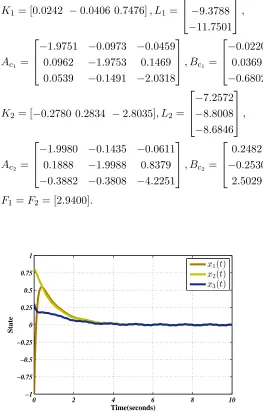
K1 = [0.0242 −0.0406 0.7476], L1 =



 

−11.5193 −9.3788 −11.7501



 ,

Ac1 =



 

−1.9751 −0.0973 −0.0459 0.0962 −1.9753 0.1469 0.0539 −0.1491 −2.0318





, Bc1 =



 

−0.0220 0.0369 −0.6802



 

K2 = [−0.2780 0.2834 −2.8035], L2 =



 

−7.2572 −8.8008 −8.6846



 ,

Ac2 =



 

−1.9980 −0.1435 −0.0611 0.1888 −1.9988 0.8379 −0.3882 −0.3808 −4.2251





, Bc2 =



 

0.2482 −0.2530

2.5029



 

F1 =F2 = [2.9400].

0 2 4 6 8 10

−1 −0.75 −0.5 −0.25 0 0.25 0.5 0.75 1

Time(seconds)

State

x₁₍t₎ x₂₍t₎ x₃₍t₎

Fig. 1: State response for closed-loop system

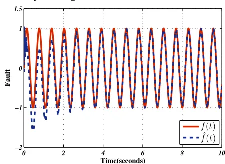
For the fault f(t) = 1.5(0.4 cos(5t) + 0.3 sin(20t))

0 2 4 6 8 10

−1 −0.75 −0.5 −0.25 0 0.25 0.5 0.75 1

Time(seconds)

State

x₁₍t₎ x₂₍t₎ x₃₍t₎

Fig. 2: State response for open-loop system

0 2 4 6 8 10

−2 −1 0 1 2

Time(seconds)

Fault

f(t) ˆ

f(t)

Fig. 3: Estimation of estimated fault with actual fault

with the initial condition [x1(0) x2(0) x3(0)]T = [−1 0.8 0.3]T and the obtained gain values, the state response of the closed-loop and open-loop system are displayed in the Fig. 1 and Fig. 2 respectively. In particular, from Fig. 1 it is obvious that the system attains stability with in 2-5 seconds even in the presence of time-varying actuator fault. It is noticed from the Fig. 3 the estimated fault tracks the original fault with maximum estimation error 0.8650, which shows the effectiveness of prescribed fault-tolerance controller. The membership function is illustrated in Fig. 4. The output response with and without fault is displayed in Fig. 5.

Suppose, the fault is taken as f(t) = sin 10(t+ 1)− 3e−10∗(t+2)2₊₁

1, then from the Fig. 6 the estimation of fault with its estimated fault also have more accuracy. By observing the simulation studies, it is obvious that

0 2 4 6 8 10 0

0.25 0.5 0.75 1

Time(seconds)

Membership function

ϕ₁ ϕ₂

Fig. 4: Membership function

0 2 4 6 8 10

−0.1 0 0.1 0.2 0.3 0.4 0.5 0.6 0.7

0.8 With fault_{Without fault}

5.6 5.8 6 −0.015

−0.01 −0.005 0 0.005 0.01

Time(seconds)

Output

Fig. 5: Output response for with fault and without fault

the dynamic-output-feedback controller can promptly re-claim performance and stability of the considered closed-loop even in the existence of disturbance and time-varying fault with precious estimation of the actuator faults.

5.Conclusion

In this paper, the problem of resilient reliable dynamic-output-feedback H∞ control for the class of T-S fuzzy

model with time varying fault and delay is investi-gated. Especially, the time-varying fault is dealt by using adaptive fault algorithm. In conjunction of L-K functional technique, S-procedure and Schur’s lemma, a set of necessary and sufficient conditions has been obtained for asymptomatic stability of T-S fuzzy delayed system in the presence of time-varying actuator fault. Finally a numerical example is given to demonstrate the

0 2 4 6 8 10

−2 −1 0 1 1.5

Time(seconds)

Fault

f(t) ˆ

f(t)

Fig. 6: Estimation of estimated fault with actual fault

effectiveness of the proposed controller.

REFERENCES

[1] Y. Liu, B.Z. Guo, J.H. Park and S. Lee. “Event-Based Reliable Dissipative Filtering for T-S Fuzzy Systems With Asynchronous Constraints”, IEEE Transactions on Fuzzy Systems, volume 26, no. 4, pages 2089-2098, 2018.

[2] Y. Wang, H. Shen and H.R. Karimi, “Dissipativity-Based Fuzzy Integral Sliding Mode Control of Continuous-Time T-S Fuzzy Systems”. IEEE Transactions on Fuzzy Systems, volume 26, no. 3, pages 1164 - 1176, 2018.

[3] X. Su, P. Shi, L. Wu, M.V. Basin. “Reliable Filtering With Strict Dissipativity for T-S Fuzzy Time-Delay Systems”. IEEE Transactions on Cybernetics, volume 44, no. 12, pages 2470 -2483, 2014.

[4] C. Peng, S. Ma, and X. Xie. “Observer-Based Non-PDC Control for Networked T-S Fuzzy Systems with an Event-Triggered Communication”. IEEE Transactions on Cybernetics, volume 47, no. 8, pages 2279 - 2287, 2017.

[5] D. Zhang, Q.L. Han and X. Jia. “Network-Based Output Track-ing Control for a Class of T-S Fuzzy Systems That Can Not Be Stabilized by Nondelayed Output Feedback Controllers”. IEEE Transactions on Cybernetics, volume 45, no. 8, pages 1511-1523, Aug. 2015.

[6] H. Li, C. Wu, S. Yin and H.K. Lam. “Observer-Based Fuzzy Control for Nonlinear Networked Systems Under Unmeasurable Premise Variables”, IEEE Transactions on Fuzzy systems, Vol. 24, no. 5, pages 1233-1245, 2016.

[7] X. Zhao, Y. Yin, L. Zhang and H. Yang. “Control of Switched Nonlinear Systems via T-S Fuzzy Modeling ”. IEEE Transac-tions on Fuzzy systems, volume 24, no. 1, pages 235-241, 2016. [8] W. Xiong, W. Yu, J. Lu and X. Yu. “Fuzzy Modelling and Consensus of Nonlinear Multiagent Systems With Variable Structure”. IEEE Transactions on Circuits and Systems, volume 61, no. 4, pages 1183-1191, 2014.

[9] O. M. Kwon, M. J. Park, J. H.Park and S.M. Lee. “Stability and stabilization of TS fuzzy systems with time-varying delays via augmented Lyapunov-Krasovskii functionals”. Information Sciences, volume 372, no. 1, pages 1-15, 2016.

[10] Z. Lian, Y. He, C.K. Zhang and M. Wu. “Stability analysis for T-S fuzzy systems with time-varying delay via free-matrix-based integral inequality”. International Journal of Control, Automation and Systems, volume 14, no. 1, pages 21-28, Feb. 2016.

[11] L. Li, M. Chadli, S.X. Ding, J. Qiu and Y. Yang, “Diagnostic Observer Design for TS Fuzzy Systems: Application to Real-Time-Weighted Fault-Detection Approach ”. IEEE Transactions on Fuzzy Systems, volume 26, no. 2, pages 805-816, April. 2018.

[12] F. You, H. Li, F. Wang and S. Guan. “Robust Fast Adaptive Fault Estimation for Systems with Time-Varying Interval De-lay”, Journal of the Franklin Institute, volume 352, no. 12 pages 5486-5513, 2015.

[13] T. Youssef, M. Chandli, H.R. Karimi and R. Wang. “Actuator and sensor faults estimation based on proportional integral observer for TS fuzzy model”. Journal of the Franklin Institute, volume 354, no. 6, pages 2524-2542, 2017.

[14] S.H. Huang and G.H. Yang. “Fault Tolerant Controller Design for TS Fuzzy Systems With Time-Varying Delay and Actuator Faults: A K-Step Fault-Estimation Approach ”. IEEE Transac-tions on Fuzzy systems, volume 22, no. 6, pages 1526-1540, 2014.

[15] H. Yang, Y. Xia and B. Liu. “Fault Detection for TS Fuzzy Discrete Systems in Finite-Frequency Domain”. IEEE Transac-tions on Systems, Man, and Cybernetics, Part B (Cybernetics), volume 41, no. 4, pages 911-920, 2011.

[16] X. J. Li and G.H. Yang. “Fault Detection in Finite Frequency Domain for Takagi-Sugeno Fuzzy Systems With Sensor Faults ”, IEEE Transactions on Cybernetics , volume 44, no. 8, pages 1446-1458, 2014.

[17] D. Ichalal, B. Marx, J. Ragot and D. Maquin. “Fault detection, isolation and estimation for TakagiSugeno nonlinear systems ”. Journal of the Franklin Institute , volume 351, no. 7, pages 3651-3676, July 2014.

[18] X. Hu, L. Wu, C. Hu, Z. Wang and H. Gao. “Dynamic output feedback control of a flexible air-breathing hypersonic vehicle via TS fuzzy approach ”. International Journal of Systems Science , volume 45, no. 8, pages 1740-1756, Aug. 2014. [19] W. Zheng, Z.M. Zhang, H.B. Wang, H.R. wang and P.H. Yin.

“Stability Analysis and Dynamic Output Feedback Control for Nonlinear T-S Fuzzy System with Multiple Subsystems and Normalized Membership Functions”. International Journal of Control, Automation and Systems, volume16, no. 6, pages 2801-2813, 2018.

[20] H. D. Choi, C. K. Ahn, P. Shi, L. Wu, M. T. Lim. “Dynamic output-feedback dissipative control for TS fuzzy systems with time-varying input delay and output constraints”. IEEE Trans-actions on Fuzzy Systems, volume 25, no. 3, pages 511 - 526, 2017.

[21] X.H. Chang, J. Xiong and J.H. Park. “Fuzzy robust

dynam-ic output feedback control of nonlinear systems with linear fractional parametric uncertainties ”. Applied Mathematics and Computation, volume 291, no. 1, pages 213-225, 2016. [22] D.H. Lee, J.B. Park, Y.H. Joo and S.K. Kim. “Local H∞

controller design for continuous-time T-S fuzzy systems”. Inter-national Journal of Control, Automation and Systems , volume 13, no. 6, pages 1499-1507, 2015.

[23] P. Shi, M. Chadli, Z. Xi and R. K. Agarwal. “Mixed H-Infinity and Passive Filtering for Discrete Fuzzy Neural Networks with Stochastic Jumps and Time Delays ”. IEEE Transactions on neural networks and learning systems, volume 27, no. 4, pages 903-909, 2016.

[24] Q. Gao, G. Feng, Z. Xi , Y. Wang and J. Qiu. “A New Design of Robust H∞ Sliding Mode Control for Uncertain

Stochastic T-S Fuzzy Time-Delay Systems”. IEEE Transactions on Cybernetics, volume 44, no. 9, pages 1556-1566, 2014.