ENHANCING THE SPEED, ACCURACY OF DEEP LEARNING USING GINI INDEX BASED FUZZY DECISION TREES

DOI: http://dx.doi.org/10.26483/ijarcs.v8i9.5053

Volume 8, No. 9, November-December 2017

International Journal of Advanced Research in Computer Science

RESEARCH PAPER

Available Online at www.ijarcs.info

ISSN No. 0976-5697

ENHANCING THE SPEED, ACCURACY OF DEEP LEARNING

USING GINI INDEX BASED FUZZY DECISION TREES

S.V.G.Reddy

Associate Professor, Dept. of CSE, GIT, GITAM University,India

Prof. K.Thammi Reddy Professor, Dept. of CSE, GIT, GITAM University,India

Prof. V.Valli Kumari Professor, Dept. of CS & SE,

college of engineering, Andhra University,India

Abstract: Deep Learning has gained tremendous importance due to its advancement in various fields of text mining, speech recognition,

computer vision, natural language processing etc. The weights of the input layer attributes and the series of hidden layers of deep learning plays a dominant role in its fast classification and accuracy. The weight adjustment algorithm for the Deep Learning is proposed in this paper. Generally, the weights can be determined by mathematical techniques, can be suggested by the domain experts or by considering random weights. In this proposed work, the weights of a neural network are computed mathematically by constructing the fuzzy decision tree. It is proposed to use the least gini index value of the attribute of the fuzzy decision tree as the weight of the corresponding attribute for the weight adjustment algorithm to classify using neural networks. Fast classification and accuracy is achieved with the computed gini weights of the deep learning which outperforms when compared with the fuzzy decision tree classifiers.

Keywords: Deep Learning, Gini index, weight, fuzzy, Decision trees, Classification Accuracy

1. INTRODUCTION

Classification is a very useful and powerful technique with which the hidden knowledge patterns can be extracted from data. There are standard ID3, C4.5 algorithms for classification purpose which uses Entropy as a splitting criterion, but the SLIQ algorithm which is applied here uses gini index as split measure. SLIQ is a decision tree classifier which can deal with both the numeric and categorical attributes. It uses a pre-sorting technique and enables to scale for large data sets irrespective of number of classes, attributes and records thus making it more significant in the data classification. There is a decision tree classifier CLOUDS [1] which creates the splitting points for the numeric attributes.

Crisp decision tree algorithms almost faces the trouble of arriving at sharp decision boundaries which can be rarely seen in the real life classification problems and hence the fuzzy decision trees which are more efficient are used in this paper. The gini index is used as the best split measure for the fuzzy decision trees. The problem with the fuzzy decision trees is, appropriate membership function cannot be identified. In fact, the previous studies / techniques proves that the fuzzy decision trees contains gradual transitions between attribute values when compared with crisp decision trees. Generally the attributes of the data set are converted in to fuzzy values using a triangular or trapezoidal membership function. In this proposed work, the fuzzy values are computed for the split values of an attribute during decision tree construction.

One of the approach to build a decision tree is by using the parameter called gini index [2]. Gini index is calculated for all the attributes at various split points and the attribute having least value of gini index is decided as the ROOT

which is considered as the Best classifier attribute. So, lot of PRIORITY & WEIGHTAGE is given for the Root attribute for classifying the records. That means the minimum / least value of gini index of an attribute tells that the records of that attribute are well distributed and would be classified with more accuracy and Hence that attribute would be decided as the ROOT of the decision tree.

On the other hand, Deep Learning is a type of Artificial neural network which contains more than one hidden layer and learns to perform the classification tasks directly from images, text, sound. The weight of an attribute of Deep Learning model can be computed using few mathematical techniques or can be suggested by the domain experts or simply using the Random weights. The proper assigning of weights of neural network leads to rapid computations and achieve more classification accuracy. In this work, it is proposed to assign the weight of attribute of neural network model mathematically by constructing fuzzy decision tree. Then the technique of applying the least value of gini index value of the attribute as the weight [3] [4] of the corresponding attribute to classify the same data set using Neural Networks is proposed in this model. Here, the proposed novel approach aims to fuzzify the decision boundary at each node of the decision tree and build an efficient neural networks model with proposed gini weights to achieve better classification accuracy. The proposed gini weights are considered and applied on various types of neural networks such as Deep Learning, Backpropagation, Multi Layer Feed Forward and good results are observed in all the cases.

construction. And section 4 stresses on the proposed methodology and illustrates the usage of gini values for the nodes of fuzzy decision tree as the weights and narrates the classification process using neural networks. Section 5 emphasizes on the various implementations using decision tree and different types of neural networks such as Deep Learning, Backpropagation, Multi Layer Feed Forward and compare the classification accuracy by giving various types of inputs.

2. SLIQ & GFDT ALGORITHM

In this approach, Fuzzified decision tree would be constructed with gini index as best split measure. So, the concept of split point, fuzzy value and gini index would be explained here. In this proposed work, the Wisconsin data set is used which contains 699 tuples. The data set consists of id, 9 attributes and a class label. There are some missing values and the preprocessing is done to obtain the complete data. The 3-fold cross validation is performed on the data set and three pairs of training and testing sets were prepared. For easy understanding, a sample data of 20 records is taken which contains attributes a1, a2, a3, class label (refer table 1).

Every attribute may contain several split points and the gini index is computed for all the attributes at all the split points. Firstly, to compute the split point, attribute, class label from the sample data is taken. And the attribute is sorted in ascending order, then due to sorting of the attribute, class label records would also be altered correspondingly. There are only two class labels 1 & 2 in the data set. Then after sorting, the class label is verified from top to bottom in each attribute list. If there is a change observed in the class label from “1 to 2” or “2 to 1”, then the corresponding attribute values related to class label 1 and class label 2(or class label 2 & class label 1) are taken and average them and their average value would be preserved as split point respectively.

Table 1 – sample data set

The split points would be computed for all the attributes (refer table 2). let’s consider attribute a2 which is computed in the following way. Column a2 is sorted, and the corresponding class label have altered. And the change in class label from “1 to 2” or “2 to 1” is verified and we can

notice two split points at (58,66) and (66,68). Randomly, let’s calculate the split point of attribute a2 at (66,68).

Here the split point would be average of 66, 68 which comes to 67.And the membership value for each record µ by default is taken as 1/c (c is the number of class labels used which are 2) which comes to 0.5. Then the standard deviation is calculated for the attribute a2 which comes to 3.451087. Table 2 – Data set, split points & fuzzy values

// The attributes sno, a1,a2,…a9, class. , m – number of attributes, n – number of records, sp - split point Function Split()

{

for( I = 1 to m ) {

sort a i for( j = 1 to n ) {

if ( ( class label [ j ] ==1 && class label [ j+1 ] ==2) ||( class label [ j ] ==2 && class label [ j+1 ] ==1))

sp [ j ] = (aj + a(j+1) ) / 2 } } }

//c - number of class labels , n – number of records Function Fuzzyvalue()

{ µ = 1/c for (i = 1 to sp ) {

x1 [ i ] = 1- 1/(1+exp( -(σ) * ( x - split point))) x2[i] = x1 [ i] * µ

}

for (i = sp to n ) {

x3 [ i ] = 1 / (1+exp( -(σ) * ( x - split point))) x4[i] = x3 [ i] * µ

Crisp decision tree algorithms almost faces the trouble of arriving at sharp decision boundaries and to overcome those problems, In this model the fuzzification [5] [6] of decision boundary at each node of the decision tree is proposed to provide gradual transitions between attribute values. For the set of above records above the split point is treated as top partition, the set of records below the split point is treated as bottom partition and the fuzzy value is computed for all the records of both top, bottom partitions.

Fuzzy value (top partition) = 1- 1/(1+exp( -(σ) * (a2-split point)))

Fuzzy value (bottom partition) = 1/(1+exp( -(σ) * (a2-split point)))

Now, let’s compute the fuzzy values for attribute a2 (refer table2). Here, the records from 58 to 66 of attribute a2 would be treated as top partition and 68 to last 69 as bottom partition. It means, x1 is computed for attribute a2 from 58 to 66 and other records it is taken as zero value. And x2 is computed for attribute a2 from 68 to last 69 and other records it is taken as zero value. And x1*µ, x2*µ are computed in the similar manner. The final fuzzy value is computed by merging both x1*µ, x2*µ. Lastly, the “sno” is sorted to get the records from 1 to the end of training data set.

Gini index / coefficient tells that “If all persons hold the same percentage of a resource, inequality is at a minimum, and If a single person holds all of a given resource, inequality is at a maximum”. That means the minimum / least value of gini index of an attribute tells that the records of that attribute are well distributed and would be classified with more accuracy.

Then the gini index is computed using the final fuzzy value f as

Gi ( split point ) =

Where p is the total number of partitions [7] , c is the total number of class labels, S is the sum of fuzzy membership values, Sp is the sum of fuzzy membership values of a partition, Spc is the sum of fuzzy membership values of a partition of a class.

From the table 2, the number of class labels c = 2, the number of partitions p =2, from the column “f”, the sum of all fuzzy values s= 9.798203799, Above the split point 67, the sum of fuzzy values Sp= 6.346317672 , and below the split point 67, the sum of fuzzy values Sp= 3.451886127. Above the split point 67, the sum of fuzzy values with class label =1, Sp1 = 4.846317672, with class label 2, Sp2 = 1.5, below the split point 67, the sum of fuzzy values with class label=1, Sp1=0, with class label 2 , Sp2= 3.451886127.

Now,gi(67)=(6.346317672/9.798203799)*(1– (4.846317672/6.346317672)2-(1.5/6.346317672)2) +(3.451886127/9.798203799)*(1-(0/3.451886127)2-(3.451886127/3.451886127)2)

= 0.648 * (1- 0.58 – 0.057) + 0.352 * (1 – 0 - 1) = 0.234 For each attribute, at every change in the class label, split points would be computed and the gini index is calculated for every split point of all the attributes. Let’s say, there are four

split points for the first attribute a1 and the gini index is computed for all the four points and pick the attribute with least value of gini index. Similarly, the gini index is calculated for all the other attributes and the least gini index value of all the attributes is picked. It means the least gini index value from all the attributes is taken and selected as the best classifier attribute and also as the ROOT of the decision tree.

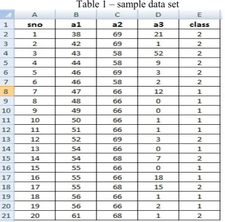
In the proposed work, using Wisconsin data set , “a3” at split point 3.5 and at 311 record with 0.1448 gini index value is chosen as ROOT which can be observed in fig 1.

3. FUZZY DECISION TREE CONSTRUCTION

The ROOT is chosen and it is required to determine the other nodes of the decision tree [8] [9] [10]. The crucial part is, how to compute the left subtree, right subtree of the Root in order to build the decision tree.

Now, from table 2, observe the values of the x1*µ, x2*µ. Firstly, lets modify the x1*µ records. Here, the values of x1*µ from 58 to 66 of a2 attribute remain the same , but from 68 to 69 of a2 attribute, the records would be replaced by (0.5- x2*µ) that is, at 68 of a2 attribute (sno 14), the x1*µ is replaced with (0.5- 0.4846318) = 0.015 and it is calculated for the other records in the similar manner.

similarly , lets modify the x2*µ records. Here the values of x2*µ from 58 to 66 of a2 attribute would be replaced by (0.5- x1*µ) , but from 68 to 69 of a2 attribute, the records remain the same. That is, at 58 of a2 attribute (sno 3), the x2*µ is replaced with (0.5- 0.5) = 0, at 66 of a2 attribute (sno 7), the x2*µ is replaced with (0.5- 0.48463177) = 0.015 and it is repeated for the other records.

Now the x1*µ and x2*µ list of values were updated. Then the updated x1*µ values are taken as the fuzzy values to compute the left node for the ROOT a3. Now, the gini index is calculated for all the attributes a1 to a9 at various split points excluding a3 (As a3 is the ROOT). Now, the attribute having least value of gini index at a split point would become the left node for ROOT “a3”. That is a6 attribute at split point 6.5 at 344 record with gini index value as 0.0759 has become theleft node for ROOT a3 which can be observed in the fig 1.

Similarly, the updated x2*µ values are taken as the fuzzy values to compute the right node for the ROOT a3. Now, the gini index is calculated for all the attributes a1 to a9 at various split points excluding a3 and a6 (As a3 is the ROOT, a6 is the left child) . Now, the attribute having least value of gini index at a split point would become the right node for ROOT “a3”. That is a2 attribute at split point 1.5 with gini index value as 0.1750 has become the right node for ROOT a3 which can be observed in the fig 1.

Fig 1 – The decision tree with Root, and other nodes with

their gini index values.

4. PROPOSED METHODOLOGY

The KEY point is, the gini index is calculated for all the attributes at various split points and the least value of gini index of an attribute is decided as the ROOT which is considered as the Best classifier attribute for the complete fuzzified decision tree. Similarly, all the other nodes of the decision tree is built using the least value of gini index as explained above in the Fuzzy decision tree section. Now, the gini index values of the nodes(attributes) of the decision tree are considered as the weight of that corresponding attributes in our proposed work.

This point is like a Bridge from Decision tree to Neural Networks which works collaboratively. That is, the results of fuzzy decision tree are taken and implemented for the neural network. That is, the least gini index values of a1,a2,a3, ...a9 attributes which are 0.1140, 0.1750, 0.1448, …0.2422 were considered as the “weights” of those corresponding attributes to classify using neural networks.

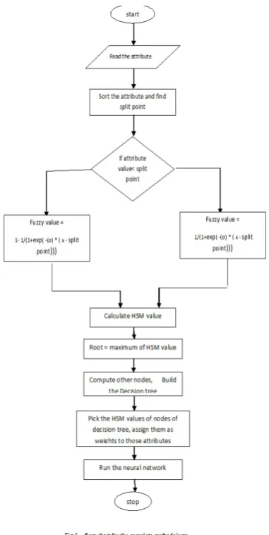
The Weight Adjustment Algorithm for the complete proposed methodology is as follows (refer fig 5) :

1. Read the data set, // 9 attributes and a class label 2. Sort an attribute and find the split point,

3. Compute the fuzzy values of attribute above the split point and below the split point,

4. Calculate the gini value of that attribute using the fuzzy values,

5. Similarly calculate the gini values for all the attributes and pick the least gini value,

6. Choose one attribute with least gini index value as the ROOT of fuzzy decision tree,

7. Similarly compute the other nodes and build the fuzzy decision tree,

8. Pick the gini values of all the nodes(attributes) of fuzzy decision tree and assign them as weights to the corresponding attributes,

9. The data set which is normalized and multiplied with gini weights are given to the different types of neural network such as Deep Learning, Backpropagation, Multi Layer Feed forward, Run

and compute the classification execution time and accuracy.

Using the above weights, the testing is done with three types of input data such as a) Wisconsin data set b) normalized Wisconsin data set, c) normalized data with gini weights (gini weighted inputs) and implemented on various types of neural networks such as Deep Learning, Backpropagation and Multi Layer Feed Forward and effective results are observed in all three cases.

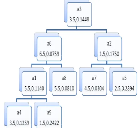
Implementation using Deep Learning

Deep Learning [11] [12] [13] [14] is gaining lot of importance in the recent times. Deep learning has become so popular in the fields of pattern recognition and computer vision etc.. Deep learning generally uses two types of networks such as convolutional neural network and Autoencoders. The Sparse Autoencoder is used for the proposed work. The network comprises of input layer, two hidden layers, softmax layer, output layer. The two hidden layers are implemented using encoders. First the hidden layers are trained in an unsupervised fashion and train the softmax layer and finally join all the hidden and softmax layers to form a deep network which is trained in a supervised fashion. The first hidden layer’s encoder reads the input and extract main features and the second hidden layer’s encoder reads the features that were extracted by the first hidden layer (encoder) and still learns the small representations (micro level features) of the input data. In fact the deep learning neural networks (refer Fig – 2) classifies the data in a most efficient way. Hence, the testing is performed by giving the normalized Wisconsin data set and gini weighted inputs to the network and verified the total execution time. It is observed that the classification efficiency is same for the two cases, but the gini weighted inputs have executed the code much faster than the normalized data. The corresponding observations are presented in Results section.

Implementation using Back Propagation neural networks Backpropagation [15] [16] is nothing but propagating the error backward, and after the adjustment of the weights, the optimal classification is achieved. In this paper, it is proposed to measure and compare the classification accuracy in three aspects. They are

1) check the classification accuracy of the data set using fuzzy decision tree,

2) check the classification accuracy of the data set by normalizing the data between 0 and 1 using neural networks, 3) check the classification accuracy for the normalized data set with the multiplied gini weights using neural networks.

//W – weight of attribute , m – number of attributes, n – number of records

Function Giniweight() {

for( i = 1 to m) {

for( j = 1 to n) {

X I j = ( j – j min ) / (j max - j min ) // normalize the data between 0 and 1

y I j = X I j * W I //gini weight is multiplied to the input attribute

The first aspect would be, the generation of the fuzzy decision tree using the train data set. Then the classification accuracy is measured by applying the test data set for the fuzzy decision tree. After generating the Rules from the fuzzy decision tree, then the test data set is given to the Rules and classification accuracy is measured and it is observed that the code is run with eight errors out of 232 test records with this fuzzy decision tree which comes to 96.55% efficiency.

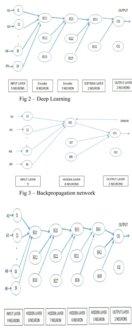
The second aspect would be, the same data set is taken, normalize the data set between 0 and 1(refer function giniweight() ) , and then classify the data using neural networks. It means, the train data, test data, and the neural network configuration file which contains “Input_Neurons, Hidden_Neurons, Output_Neurons, Learning Rate, Momentum, Train_Input_Records, Train_Output_Records, No_of_Iteration” are given to the neural network code, run it, and measure the classification accuracy. Regarding the neural networks, the multi layer(Input layer, hidden layer, output layer) neural network model(refer fig (3)) with back propagation is considered. The input layer comprises of 9 neurons, hidden layer of 8 neurons and the output layer with 3 neurons and learning rate of 0.25 ,the momentum of 0.9 is considered and the training, testing records, number of iterations are given to the neural network model. The input layer is given with the 9 attributes of the normalized data set, and the output layer gives an output of 001(1) or 010(2) to three neurons where (001)1 is benign and (010)2 is malignant. The sigmoid Activation function ( 1/ (1+e(-x)) ) is used in our model where x is the linear function of weight, attribute and the bias. The error is calculated at the output layer and it is shared back to the neurons of the model using the concept of back propagation. It is observed that the code is run with four errors out of 232 test records with the neural networks which comes to 98.27% accuracy.

The third aspect would be, the same data set is taken, normalize the data set between 0 and 1 and multiply with the gini weights (refer function giniweight() ), and then classify the data using neural networks with back propagation as it is done in the second aspect . It means, the train data, test data, and the neural network configuration file are given to the neural network code and measure the classification accuracy. It is observed that the code is run with three errors out of 232 test records with the neural networks which comes to 98.7% accuracy which is a biggest improvement of the classification accuracy .

Implementation using Multi Layer Feed Forward neural networks

The network which does not contain cycles or the feedback loops is called a feed forward neural network. Here, the network comprises of input layer, hidden layer and output layer. The testing is done using the Wisconsin data set, normalized Wisconsin data set and gini weighted inputs on the network comprising of single, two, three and four hidden layers (refer Fig – 4) and got good results in all the cases. The gini index is computed using the final fuzzy value [17] Please refer Results.

5. RESULTS

The Results related to the Deep Learning, Backpropagation and Multi Layer Feed Forward neural networks are illustrated in the following.

Deep Learning

When the different forms of input data(as explained above) are given to the Deep Learning, the Results are in the following manner (Refer table 3, Fig 6) and the execution speed is increased by 150%.

Fig 2 – Deep Learning

Fig 3 – Backpropagation network

Fig 5 – flow chart for the complete methodology

Table 3 – Execution time of Deep Learning

Implementation Total time of Execution(seconds)

Normalized Wisconsin

data set 6.3 ± 0.1 Gini weighted inputs 2.5 ± 0.1

Fig 6 – Deep Learning execution time

Back Propagation neural networks

When the different forms of input data(as explained above) are given to the Backpropagation neural network, the Results are in the following manner (refer table 4, Fig 7 ).

Table 4 – classification accuracy of decision tree & neural networks

Sno Description of the implementation Classification _Accuracy

1 Wisconsin Data set using Decision _tree 96.5%

2

Wisconsin Data set which is normalized and using neural

networks 98.2%

3 Wisconsin Data set which is normalized and multiplied with

gini weights using neural networks 98.7%

Fig 7 – Backpropagation Neural Network Classification Accuracy

Multi Layer Feed Forward neural networks

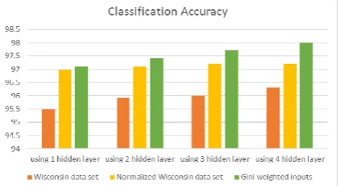
When the different forms of input data(as explained above) are given to the Multi Layer Feed Forward neural networks with different number of hidden layers, the Results are in the following manner. (Refer table 5, Fig 8)

Table 5 – classification accuracy of Multi Layer Feed Forward neural network

Implementation Using 1 Classification Accuracy Hidden

layer

Using 2 Hidden layers

Using 3 Hidden layers

Using 4 Hidden layers Wisconsin data

set 95.5 95.9 96 96.3 Normalized

Wisconsin data set

97 97.1 97.2 97.2

Gini weighted

Fig 8 – Multi Layer Feed Forward Neural Network Classification Accuracy

6. CONCLUSION

The fuzzy decision tree is constructed using gini index as the best split measure. To enhance the speed & accuracy of the classification using neural networks , the least gini index value of each attribute is taken as the Weight of the corresponding attribute for the weight adjustment algorithm and tested using Deep Learning, Backpropagation, Multi Layer Feed Forward neural networks and achieved very good results. And as a future work, there are few parameters like Information gain, HSM which plays a dominant role in the classification of the data using various supervised learning algorithms and the values of those parameters can be taken as the weight and compare all the parameters and choose the one which would give the best classification accuracy. Even the genetic algorithm can be applied to suggest the best optimal parameter to derive the weights.

7. ACKNOWLEDGEMENT

I am very much thankful to my supervisor Prof.K.Thammi Reddy, my co supervisor Prof. V.Valli Kumari for their guidance and constant monitoring of my PhD work.

REFERENCES

[1] Alsabti, K., Ranka, S., & Singh, V. (1998). CLOUDS: A decision tree classifier for largedatasets. In Knowledge discovery and data mining (pp. 2–8),

[2] B.chandra, P.Paul Varghese, fuzzifying gini index based decision trees, Elsevier ( Expert systems with applications 36 (2009), pp 8549 - 8559 ,

[3] Chandra, B., & Paul, P. (2007). On improving the efficiency of SLIQ decision tree algorithm. In Proceedings of IEEE international joint conference on neural networks, IJCNN – 2007,

[4] Manish Mehta, Rakesh Agrawal and Jorma Rissanen. SLIQ: A Fast Scalable Classifier for Data Mining, Advances in Database Technology — EDBT '96. EDBT 1996. Lecture Notes in Computer Science, vol 1057. Springer, Berlin, Heidelberg,

[5] Adamo, J. M. (1980). Fuzzy decision trees. Fuzzy Sets and Systems, 4, 207–219,

[6] Cristina, O., & Wehenkel, L. (2003). A complete fuzzy decision tree technique. Fuzzy Sets and Systems, 138, 221– 254,

[7] Chengming, Q. (2007). A new partition criterion for fuzzy decision tree algorithm. In Intelligent information technology application, workshop on 2–3 December 2007 (pp. 43–46), [8] Breiman, L., Friedman, J. H., Olshen, J. A., & Stone, C. J.

(1984). Classification and regression trees. Belmont, CA: Wadsworth International Group, open journal of geology, 2016, vol 6, no 7 ,

[9] Chandra, B., Mazumdar, S., Arena, V., & Parimi, N. (2002). Elegant decision tree algorithms for classification in data mining. In Proceedings of the 3rd international conference on information systems engineering (workshops), IEEE ,CS (pp. 160–169),

[10] Chandra, B., & Paul, P. (2006). In Robust algorithm for classification using decision trees CIS-RAM 2006 (pp. 608– 612). IEEE,

[11] Jürgen Schmidhuber, Deep Learning in neural networks: An Overview, Elsevier(Neural networks), 2015, vol 61, p 85-117, [12] Victoria j hodge, simon o keefe, jim Austin, Hadoop neural

network for parallel and distributed feature selection, Elsevier(Neural networks), 2016, vol 78, p 24-35,

[13] Jihun kim, jong hong kim, gil-jin jang, minho lee, fast learning method for convolutional neural networks using extreme learning machine and its application to lane detection, Elsevier(Neural networks), 2017, vol 87, p 109-121,

[14] https://in.mathworks.com/help/nnet/examples/training-a-deep-neural-network-for-digit-classification.html

[15] M.W.Gardner, S.R.Dorling, Artificial neural networks (the multilayer perceptron)—a review of applications in the atmospheric sciences, Elsevier, Atmospheric environment, 1998, pp 2627 – 2636,

[16] Bing Cheng, D.M.Titterington, Neural Networks: A Review from a Statistical Perspective, Statistical Science Volume 9, Number 1 (1994), p2-30.